Captum: Explain/Interpret Predictions Of PyTorch Networks
PyTorch is one of the most preferred Python Deep learning libraries for designing neural networks by researchers and ML engineers worldwide. It provides a lot of features to handle tabular data, text data, image data, audio data, video data, etc. It's even faster compared to other libraries and default settings generally give good results. With the rise of data and complicated deep neural networks, it has become hard to interpret predictions made by networks. Traditional ML algorithms (decision tree, gradient boosting machines, random forests, etc.) were quite easy to understand and interpret but they are not good for unstructured data like images, text, audio, video, etc. Deep neural networks give a wonderful performance with unstructured data, but networks nowadays consist of different kinds of layers and are so deep that it is hard to interpret them. To solve this problem, over time, many algorithms have been developed for explaining/interpreting predictions of black-box ML models (deep neural networks). Many Python libraries (LIME (Local Interpretable Model-Agnostic Explanations), SHAP (SHapley Additive exPlanations), Eli5, etc.) are also developed to create visualizations explaining predictions made by the network.
As a part of this tutorial, we are going to concentrate on a new Python library named Captum which is specifically designed to explain/interpret predictions of PyTorch Networks. We'll demonstrate with simple examples how we can use Captum. We have explained the usage of Captum on tabular data as a part of this tutorial. We have separate tutorials for image and text data as well. This tutorial will help individuals get started with the library. Captum provides an implementation of many interpretation algorithms and will keep adding new algorithms as they surface.
Captum divides the algorithms that it provides for interpreting predictions into three main categories.
- Primary Attribution - Algorithms falling in this category evaluate how each individual feature contributes to prediction (output of the model). (Input Features --> Prediction)
- Layer Attribution - Algorithms falling in this category evaluates how each individual activation of the selected layer contributes to prediction (output of the model). (Layer Activations --> Prediction)
- Neuron Attribution - Algorithms falling in this category evaluates how each individual input feature contributes to the activation of a particular hidden neuron. (Input Features --> Neuron Activation)
Below, we have included a table showing a list of algorithms that Captum currently provides.
List of Algorithms for Explaining Predictions
| Primary Attribution | Layer Attribution | Neuron Attribution |
|---|---|---|
| Integrated Gradients | Layer Integrated Gradients | Neuron Integrated Gradients |
| Gradient SHAP | Layer GradientSHAP | Neuron GradientSHAP |
| DeepLIFT | Layer DeepLIFT | Neuron DeepLIFT |
| DeepLIFT SHAP | Layer DeepLIFT SHAP | Neuron DeepLIFT SHAP |
| Guided Grad-CAM | Grad-CAM | Neuron Gradient |
| Feature Ablation | Layer Feature Ablation | Neuron Feature Ablation |
| Guided Backpropagation and Deconvolution | Internal Influence | Neuron Guided Backpropagation and Deconvolution |
| Saliency | Layer Conductance | Neuron Conductance |
| Input X Gradient | Layer Gradient X Activation | |
| Feature Permutation | Layer Activation | |
| Occlusion | ||
| Shapley Value Sampling | ||
| LIME | ||
| KernelSHAP |
Installation
- !pip install captum
Below, we have listed important sections of tutorial to give an overview of the material covered.
Important Sections Of Tutorial
- Regression
- Load Dataset
- Normalize Data
- Define PyTorch Network
- Train Network
- Evaluate Network Performance
- Explain Network Predictions using CAPTUM
- Primary Attribution
- Integrated Gradients
- Feature Ablation
- Layer Attribution
- Layer Integrated Gradients
- Layer Feature Ablation
- Neuron Attribution
- Neuron Integrated Gradients
- Neuron Feature Ablation
- Primary Attribution
- Classification
- Load Dataset
- Normalize Data
- Define PyTorch Network
- Train Network
- Evaluate Network Performance
- Explain Network Predictions using CAPTUM
Below, we have imported the necessary Python library and printed the versions that we have used in our tutorial.
import torch

print("PyTorch Version : {}".format(torch.__version__))
import captum

print("CAPTUM Version : {}".format(captum.__version__))
1. Regression 
In this section, we have solved a simple regression task of predicting housing prices in California using the PyTorch network. Then, we have tried to explain the contributions of various features in predicting housing prices using Captum.
Load Dataset
In this section, we have loaded California housing dataset available from scikit-learn. The input data has 8 features (median income, house age, average rooms, average bedrooms, population, average household members, latitude, and longitude) and the target variable is median house price in hundreds of thousands of dollars. After loading the dataset, we have divided it into the train (80%) and test (20%) sets. Then, we have converted datasets to torch tensors.
from sklearn import datasets
from sklearn.model_selection import train_test_split

data_reg = datasets.fetch_california_housing()
X, Y = data_reg.data, data_reg.target

X_train_reg, X_test_reg, Y_train_reg, Y_test_reg = train_test_split(X, Y, train_size=0.8, random_state=123)

n_features_reg = X_train_reg.shape[1]

X_train_reg, X_test_reg = torch.tensor(X_train_reg, dtype=torch.float32), torch.tensor(X_test_reg, dtype=torch.float32)
Y_train_reg, Y_test_reg = torch.tensor(Y_train_reg, dtype=torch.float32), torch.tensor(Y_test_reg, dtype=torch.float32)

X_train_reg.shape, X_test_reg.shape, Y_train_reg.shape, Y_test_reg.shape
Normalize Data
In this section, we have normalized our data so that optimizer converges faster. To normalize data, We have taken the mean and standard deviation of features first. Then, we subtracted the mean from the datasets and divided them by standard deviation.
mean = X_train_reg.mean(axis=0)
std = X_train_reg.std(axis=0)

X_train_reg = (X_train_reg - mean)/ std
X_test_reg = (X_test_reg - mean)/ std
Define PyTorch Network
In this section, we have defined a simple neural network of 4 dense layers that we'll use for our classification task. The dense layers have 5, 10, 15, and 1 output units respectively. The relu activation function is applied to the output of the first three layers during the forward pass.
After defining the network, we initialized it and performed a forward pass through it to make sure that the network works as expected.
If you are someone who is new to PyTorch and want to learn how to design neural networks using it then we recommend that you go through the below link. It'll help you get started with the library.
from torch import nn
from torch.nn import functional as F

class Regressor(nn.Module):
    def __init__(self):
        super(Regressor, self).__init__()
        self.lin1 = nn.Linear(n_features_reg, 5)
        self.lin2 = nn.Linear(5, 10)
        self.lin3 = nn.Linear(10, 15)
        self.lin4 = nn.Linear(15,1)

    def forward(self, X_batch):
        layer_out = F.relu(self.lin1(X_batch))
        layer_out = F.relu(self.lin2(layer_out))
        layer_out = F.relu(self.lin3(layer_out))

        return self.lin4(layer_out).ravel()

regressor = Regressor()

preds = regressor(X_train_reg[:5])

preds
Train Network
In this section, we have trained our network. To train the network, we have defined a simple function. The function takes the model, loss function, optimizer, train data (X, Y), and a number of epochs as input. It executes a training loop number of epochs time. For each epoch, it performs a forward pass to make predictions, calculates loss, calculates gradients, and updates network parameters using gradients. The function also prints loss after the completion of epochs.
def TrainModel(model, loss_func, optimizer, X, Y, epochs=500):
    for i in range(epochs):
        preds = model(X) ## Make Predictions by forward pass through network

        loss = loss_func(preds, Y) ## Calculate Loss

        optimizer.zero_grad() ## Zero weights before calculating gradients
        loss.backward() ## Calculate Gradients
        optimizer.step() ## Update Weights

        if i % 100 == 0: ## Print Loss every 10 epochs
            print("Loss : {:.2f}".format(loss))
Below, we have trained our network using the training routine we defined in the previous cell. We have initialized a number of epochs to 2500 and the learning rate to 0.001. Then, we have initialized our regression model, mean squared error loss, and Adam optimizer. At last, we have called our training routine with the necessary parameters to perform training. We can notice from the loss value getting printed after each epoch that our network is doing a good job.
from torch.optim import SGD, RMSprop, Adam

torch.manual_seed(42) ##For reproducibility.This will make sure that same random weights are initialized each time.

epochs = 2500
learning_rate = torch.tensor(1e-3) # 0.001

regressor = Regressor()
mse_loss = nn.MSELoss()
optimizer = Adam(params=regressor.parameters(), lr=learning_rate)

TrainModel(regressor, mse_loss, optimizer, X_train_reg, Y_train_reg, epochs=epochs)
Evaluate Network Performance
In this section, we have evaluated the performance of our network on the regression task by calculating R^2 score on test predictions. We can notice from the score that it's above average and now we can try to interpret predictions of the network.
Here, we calculated R^2 score using the function available from scikit-learn. The sklearn provides many ML metrics. Please check the below link if you are interested in learning about them.
from sklearn.metrics import r2_score

test_preds = regressor(X_test_reg)
print("Test  R^2 Score : {:.2f}".format(r2_score(test_preds.detach().numpy().squeeze(), Y_test_reg.detach().numpy())))
Explain Network Predictions using CAPTUM 
In this section, we'll explain the prediction made by our trained network on individual examples. We'll try to explain a few algorithms per three different categories (Primary attribution, Layer attribution, and Neuron attribution) of Captum. The algorithms are available through 'attr' sub-module of Captum library.
Please make a NOTE that we have not explained how the algorithms work internally. We have explained how you can use them to interpret predictions. Please feel free to check algorithms research papers if you are interested in theoretical parts.
1. Primary Attribution
In this section, we have tried to interpret network predictions using primary attribution algorithms available from captum. These algorithms as we explained earlier try to find the contribution of an individual feature to prediction. We'll first find our contribution of features on prediction and then will visualize them using matplotlib.
Integrated Gradients
In this section, we have explained prediction using integrated gradients algorithm. In order to explain predictions using Captum, we first need to create an instance of an algorithm by passing the model to it and then call attribute() method of algorithm instance to generate explanations. The attribute() method accepts a batch of examples and generates an explanation for each of them.
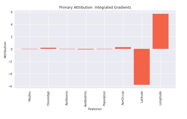
Below, we have first created an instance of IntegratedGradients() with our regressor and then called attribute() method on it with the first test example. The output is the contribution of features towards prediction. We have then visualized contributions using matplotlib. We can notice from the visualization that features like longitude, average occupancy, and average age are positively contributing to prediction whereas 'latitude' contributes negatively. The contribution of the other features seems negligible.
from captum import attr

interpreter = attr.IntegratedGradients(regressor)

interpreter
attributions = interpreter.attribute(X_test_reg[:1])

attributions
import matplotlib.pyplot as plt
import matplotlib

with matplotlib.style.context("seaborn"):
    plt.figure(figsize=(10,5))
    plt.bar(range(n_features_reg), attributions.flatten(), width=0.85, color="tomato");
    plt.xticks(range(n_features_reg), data_reg.feature_names, rotation=90)
    plt.xlabel("Features");
    plt.ylabel("Attribution");
    plt.title("Primary Attribution: Integrated Gradients");
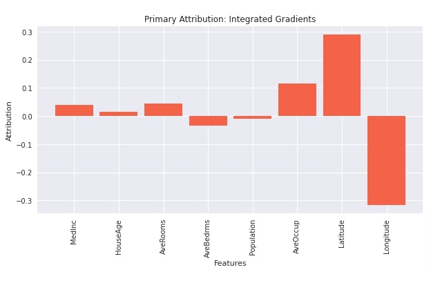
In the below cell, we have found the contribution of features on all test examples. Please be aware that running this step on a big dataset can take a long time. After generating contributions, we have taken the average of them and plotted them. We can notice from the visualization that features like 'latitude', 'average occupancy', 'average rooms', 'house age' and 'median income' contributes positively whereas 'average bed rooms', 'population' and 'longitude' negatively contributes to prediction.
from captum import attr

interpreter = attr.IntegratedGradients(regressor)
attributions = interpreter.attribute(X_test_reg)

attributions.shape
import matplotlib.pyplot as plt
import matplotlib

with matplotlib.style.context("seaborn"):
    plt.figure(figsize=(10,5))
    plt.bar(range(n_features_reg), attributions.mean(axis=0), width=0.85, color="tomato");
    plt.xticks(range(n_features_reg), data_reg.feature_names, rotation=90)
    plt.xlabel("Features");
    plt.ylabel("Attribution");
    plt.title("Primary Attribution: Integrated Gradients");
Feature Ablation
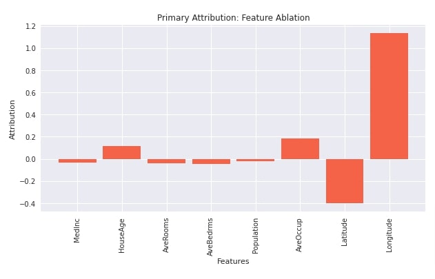
In this section, we have explained network prediction using Feature Ablation algorithm. We have first initialized the algorithm from captum with our network. Then, we have called attribute() method on it with the first test example to generate feature contributions towards prediction. Then, we have created a visualization showing feature contribution toward prediction. We can notice from the visualization that features like 'longitude', 'average occupancy', and 'house age' contributes positively to prediction whereas features like 'median income', 'average rooms', 'average bed rooms', 'population' and 'latitude' contributes negatively to prediction.
from captum.attr import FeatureAblation

interpreter = FeatureAblation(regressor)

interpreter
attributions = interpreter.attribute(X_test_reg[:1])

attributions
import matplotlib.pyplot as plt
import matplotlib

with matplotlib.style.context("seaborn"):
    plt.figure(figsize=(10,5))
    plt.bar(range(n_features_reg), attributions.flatten(), width=0.85, color="tomato");
    plt.xticks(range(n_features_reg), data_reg.feature_names, rotation=90)
    plt.xlabel("Features");
    plt.ylabel("Attribution");
    plt.title("Primary Attribution: Feature Ablation");
2. Layer Attribution
In this section, we have explained how we can use layer attribution algorithms. As we have said earlier, the algorithm in this section helps us understand how individual activation of a selected layer contributes to prediction. The layer attribution algorithms start with 'Layer' string.
Layer Integrated Gradients
In this section, we have explained how we can use Layer integrated gradients algorithm. When using layer attribution algorithms, we need to provide layer references for which we want to find out contributions.
In our case, we have first retrieved all layers of the network by calling children() method on it.
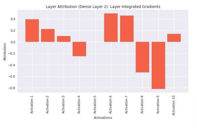
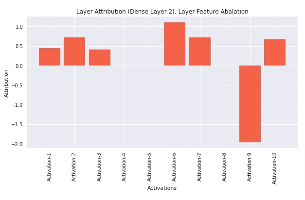
Next, when creating an instance of LayerIntegratedGradients algorithm, we need to provide a layer reference. We have provided the second layer of our network as we want to know how neurons of that layer are contributing to prediction. After initializing the algorithm, we have called attribute() method on it with the first test example to generate neuron contributions. We can notice from the output that it has generated 10 attributions which are the same as the number of output units of the second linear layer.
At last, we have visualized the contributions of individual neurons toward predictions. We can notice from the visualization that neurons 1,2,3,6,7 and 10 contribute positively to prediction whereas other neurons contribute negatively.
layers = list(regressor.children())

layers
from captum.attr import LayerIntegratedGradients

interpreter = LayerIntegratedGradients(regressor, layers[1])
attributions = interpreter.attribute(X_test_reg[:1])

attributions
import matplotlib.pyplot as plt
import matplotlib

with matplotlib.style.context("seaborn"):
    plt.figure(figsize=(10,5))
    plt.bar(range(10), attributions.flatten(), width=0.85, color="tomato");
    plt.xticks(range(10), ["Activation-{}".format(i+1) for i in range(10)], rotation=90)
    plt.xlabel("Activations");
    plt.ylabel("Attribution");
    plt.title("Layer Attribution (Dense Layer 2): Layer Integrated Gradients");
Layer Feature Ablation
In this section, we have explained network prediction using Layer Feature Ablation algorithm. We first initialized the algorithm by creating an instance of LayerFeatureAblation from captum and then called attribute() method on it with the first test instance to generate contributions of neurons. In this case, also, we are generating contributions of neurons of the second linear layer towards predictions. We have also plotted visualization showing which neurons contribute positively and which negatively.
from captum.attr import LayerFeatureAblation

interpreter = LayerFeatureAblation(regressor, layers[1])
attributions = interpreter.attribute(X_test_reg[:1])

attributions
import matplotlib.pyplot as plt
import matplotlib

with matplotlib.style.context("seaborn"):
    plt.figure(figsize=(10,5))
    plt.bar(range(10), attributions.flatten(), width=0.85, color="tomato");
    plt.xticks(range(10), ["Activation-{}".format(i+1) for i in range(10)], rotation=90)
    plt.xlabel("Activations");
    plt.ylabel("Attribution");
    plt.title("Layer Attribution (Dense Layer 2): Layer Feature Abalation");
3. Neuron Attribution
In this section, we have explained how to use Neuron Attribution algorithms for an explanation. As we had explained earlier, these algorithms let us explain how individual features of input data contribute to the activation of a particular neuron. The neuron attribution algorithms start with 'Neuron' string.
Neuron Integrated Gradients
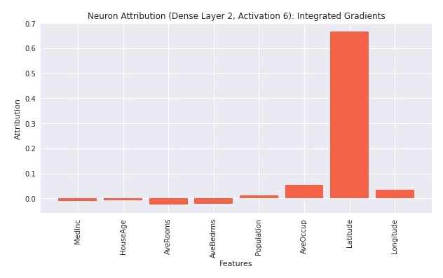
In this section, we have explained the usage of Neuron Integrated Gradients algorithm. We have first created an instance of an algorithm using NeuronIntegratedGradients() constructor. We have provided our regression model and second linear layer to the constructor. Then, we have called attribute() method on the algorithm with the first test example. We have provided 5 as a value of neuron_selector parameter. This indicates that we want to see contributions of features to the 6th neuron (indexing starts at 0) of the second linear layer. If the layer output is 3D/4D like that of Conv1D/Conv2D layers then we can provide a tuple of values to specify a particular neuron. After generating feature contributions, we have also plotted them. We can notice from the visualization that features like 'population', 'average occupancy', 'latitude', and 'longitude' contributes positively to neuron activation whereas other features ('median income', 'house age', 'average rooms', 'average bed rooms') contributes negatively.
layers = list(regressor.children())

layers
from captum.attr import NeuronIntegratedGradients

interpreter = NeuronIntegratedGradients(regressor, layers[1])
attributions = interpreter.attribute(X_test_reg[:1], neuron_selector=5)

attributions
import matplotlib.pyplot as plt
import matplotlib

with matplotlib.style.context("seaborn"):
    plt.figure(figsize=(10,5))
    plt.bar(range(n_features_reg), attributions.flatten(), width=0.85, color="tomato");
    plt.xticks(range(n_features_reg), data_reg.feature_names, rotation=90)
    plt.xlabel("Features");
    plt.ylabel("Attribution");
    plt.title("Neuron Attribution (Dense Layer 2, Activation 6): Integrated Gradients");
Neuron Feature Ablation
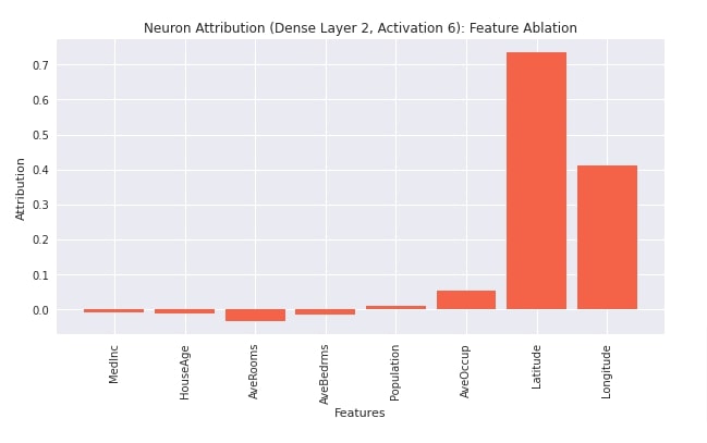
In this section, we have explained the usage of neuron feature ablation algorithm. We have created an instance of an algorithm using NeuronFeatureAblation() constructor. We have provided the regressor model and a second linear layer to the constructor. Then, we have called attribute() method with the first test example and 6th neuron index. After generating feature contributions, we have also plotted them for reference purposes.
from captum.attr import NeuronFeatureAblation

interpreter = NeuronFeatureAblation(regressor, layers[1])
attributions = interpreter.attribute(X_test_reg[:1], neuron_selector=5)

attributions
import matplotlib.pyplot as plt
import matplotlib

with matplotlib.style.context("seaborn"):
    plt.figure(figsize=(10,5))
    plt.bar(range(n_features_reg), attributions.flatten(), width=0.85, color="tomato");
    plt.xticks(range(n_features_reg), data_reg.feature_names, rotation=90)
    plt.xlabel("Features");
    plt.ylabel("Attribution");
    plt.title("Neuron Attribution (Dense Layer 2, Activation 6): Feature Ablation");
2. Classification 
In this section, we have explained how we can use various interpretation algorithms available from Captum for classification tasks. We have created a simple neural network for breast cancer classification dataset.
Load Dataset
In this section, we have loaded breast cancer dataset that we are going to use for our task. The dataset has 30 features (various measures of tumor). The target variable is a binary specifying whether a tumor is malignant or benign. The dataset is available from scikit-learn. After loading the dataset, we have divided it into the train (90%) and test (10%) sets. Then, we have wrapped datasets in torch tensors because PyTorch networks work on them only.
import numpy as np

data_classif = datasets.load_breast_cancer()
X, Y = data_classif.data, data_classif.target

X_train_classif, X_test_classif, Y_train_classif, Y_test_classif = train_test_split(X, Y, train_size=0.9, stratify=Y, random_state=123)

n_features_classif = X_train_classif.shape[1]
classes = np.unique(Y)
n_classes = len(classes)

X_train_classif, X_test_classif = torch.tensor(X_train_classif, dtype=torch.float32), torch.tensor(X_test_classif, dtype=torch.float32)
Y_train_classif, Y_test_classif = torch.tensor(Y_train_classif, dtype=torch.long), torch.tensor(Y_test_classif, dtype=torch.long)

X_train_classif.shape, X_test_classif.shape, Y_train_classif.shape, Y_test_classif.shape
n_features_classif, classes, data_classif.target_names
Define PyTorch Network
Here, we have defined a network that we'll use for our classification task. The network consists of 4 linear layers with output units 5,10,15, and 2 respectively. The first three layers apply relu activation to the output whereas the fourth layer applies softmax activation to the output to return probabilities.
After defining the network, we initialized it and performed a forward pass with a few train examples for verification purposes.
from torch import nn
from torch.nn import functional as F

class Classifier(nn.Module):
    def __init__(self):
        super(Classifier, self).__init__()
        self.lin1 = nn.Linear(n_features_classif, 5)
        self.lin2 = nn.Linear(5, 10)
        self.lin3 = nn.Linear(10, 15)
        self.lin4 = nn.Linear(15, n_classes)

    def forward(self, X_batch):
        x = F.relu(self.lin1(X_batch))
        x = F.relu(self.lin2(x))
        x = F.relu(self.lin3(x))
        x = self.lin4(x)

        return F.softmax(x, dim=1)

classifier = Classifier()

preds = classifier(X_train_classif[:5])

preds
Train Network
In this section, we have trained our network. We have set the number of epochs to 2000 and the learning rate to 0.01. Then, we have initialized our classification network, negative log loss loss function, and Adam optimizer. At last, we have called our training routine to perform the training process with the necessary parameters. We can notice from the loss values getting printed after each epoch that our network is doing a good job at the given classification task.
from torch.optim import Adam

torch.manual_seed(42) ##For reproducibility.This will make sure that same random weights are initialized each time.

epochs = 2000
learning_rate = torch.tensor(1e-2) # 0.01

classifier = Classifier()
nll_loss = nn.NLLLoss()
optimizer = Adam(params=classifier.parameters(), lr=learning_rate)

TrainModel(classifier, nll_loss, optimizer, X_train_classif, Y_train_classif, epochs=epochs)
Evaluate Network Performance
In this section, we have evaluated the performance of our network by calculating accuracy score, classification report (precision, recall, and f1-value per target class) and confusion matrix metrics on test predictions. We can notice from the test accuracy score that our network is doing a great job at the classification task.
We have calculated these metrics using the function available from scikit-learn. Please feel free to check the below link if you need more details on metrics.
from sklearn.metrics import accuracy_score, classification_report, confusion_matrix

classifier.eval()
test_preds = classifier(X_test_classif) ## Make Predictions on test dataset
test_preds = torch.argmax(test_preds, axis=1) ## Convert Probabilities to class type

print("Test  Accuracy : {:.2f}".format(accuracy_score(Y_test_classif, test_preds)))
print("\nTest Data Classification Report : ")
print(classification_report(Y_test_classif, test_preds))
print("\nConfusion Matrix : ")
print(confusion_matrix(Y_test_classif, test_preds))
Explain Network Predictions using CAPTUM 
Now, we'll explain predictions made by our classification network using various algorithms available from Captum. Like the regression section, we'll explain a few algorithms per algorithms category.
1. Primary Attribution
In this section, we have explained the usage of interpretation algorithms from primary attribution algorithms category. As discussed earlier, algorithms in this category let us find out the contributions of input data features towards the final prediction.
Integrated Gradients
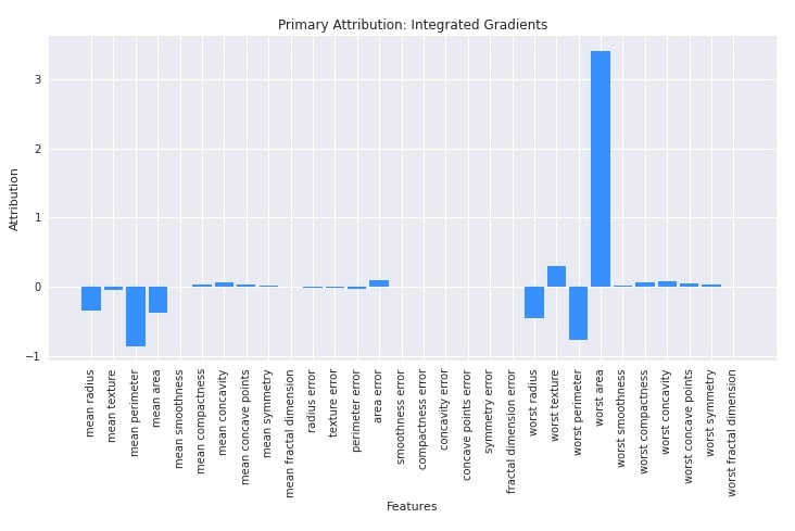
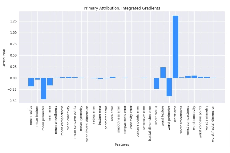
Here, we have explained the usage of integrated gradients algorithm. We have initialized algorithm using IntegratedGradients() constructor available from attr sub-module of captum library. We have provided our classification network to the constructor. After initializing the algorithm, we have called attribute() method on it with the first test example and its label to generate features contributions. Later on, we plotted a bar chart using matplotlib to show feature contribution. We can notice from the chart that features like 'worst area', 'area error', 'worst texture', 'worst compactness', 'worst concavity', 'worst symmetry', etc are contributing positively towards predictions whereas features like 'mean radius', 'mean perimeter', 'mean area', 'worst radius', 'worst perimeter', etc are contributing negatively towards prediction.
Please make a NOTE that we can provide a target label for models that generate more than one output (probabilities) per example.
from captum import attr

interpreter = attr.IntegratedGradients(classifier)
attributions = interpreter.attribute(X_test_classif[:1], target=Y_test_classif[:1])

attributions
import matplotlib.pyplot as plt
import matplotlib

with matplotlib.style.context("seaborn"):
    plt.figure(figsize=(12,5.5))
    plt.bar(range(n_features_classif), attributions.flatten(), width=0.85, color="dodgerblue");
    plt.xticks(range(n_features_classif), data_classif.feature_names, rotation=90)
    plt.xlabel("Features");
    plt.ylabel("Attribution")
    plt.title("Primary Attribution: Integrated Gradients");
Below, we have generated feature contributions for all test examples. Then, we plotted average contributions. The feature contributions almost look the same as earlier with minor changes.
from captum import attr

interpreter = attr.IntegratedGradients(classifier)
attributions = interpreter.attribute(X_test_classif, target=Y_test_classif)

attributions.shape
import matplotlib.pyplot as plt
import matplotlib

with matplotlib.style.context("seaborn"):
    plt.figure(figsize=(12,5.5))
    plt.bar(range(n_features_classif), attributions.mean(axis=0), width=0.85, color="dodgerblue");
    plt.xticks(range(n_features_classif), data_classif.feature_names, rotation=90)
    plt.xlabel("Features");
    plt.ylabel("Attribution")
    plt.title("Primary Attribution: Integrated Gradients");
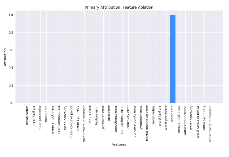
Feature Ablation
In this section, we have explained the usage of feature ablation algorithm. We have initialized algorithms using FeatureAblation() constructor. After initializing the algorithm, we have called attribute() method on it with the first test example to generate feature contributions. We have then plotted feature contributions as well.
from captum import attr

interpreter = attr.FeatureAblation(classifier)
attributions = interpreter.attribute(X_test_classif[:1], target=Y_test_classif[:1])

attributions
import matplotlib.pyplot as plt
import matplotlib

with matplotlib.style.context("seaborn"):
    plt.figure(figsize=(12,5.5))
    plt.bar(range(n_features_classif), attributions.mean(axis=0), width=0.85, color="dodgerblue");
    plt.xticks(range(n_features_classif), data_classif.feature_names, rotation=90)
    plt.xlabel("Features");
    plt.ylabel("Attribution")
    plt.title("Primary Attribution: Feature Ablation");
2. Layer Attribution
In this section, we have explained network predictions using algorithms available from layer attribution category. As discussed earlier, the algorithms in this category let us find out the contributions of individual activations of a selected layer towards the final prediction.
Layer Integrated Gradients
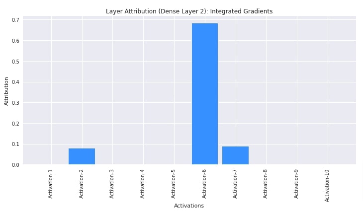
In this section, we have explained the usage of layer integrated gradients algorithm. We have created an algorithm using LayerIntegratedGradients() constructor giving it our classification network and second linear layer as input. Then, we have generated contributions of activations of the second layer towards the prediction of the first test example using the attribute() method. The second layer has 10 output units hence there are 10 contributions generated. At last, we have plotted contributions. The figure shows that activations 3,6 and 7 are contributing positively towards prediction.
layers = list(classifier.children())

layers
from captum import attr

interpreter = attr.LayerIntegratedGradients(classifier, layers[1])
attributions = interpreter.attribute(X_test_classif[:1], target=Y_test_classif[:1])

attributions
import matplotlib.pyplot as plt
import matplotlib

with matplotlib.style.context("seaborn"):
    plt.figure(figsize=(12,5.5))
    plt.bar(range(10), attributions.mean(axis=0), width=0.85, color="dodgerblue");
    plt.xticks(range(10), ["Activation-{}".format(i+1) for i in range(10)], rotation=90)
    plt.xlabel("Activations");
    plt.ylabel("Attribution")
    plt.title("Layer Attribution (Dense Layer 2): Integrated Gradients");
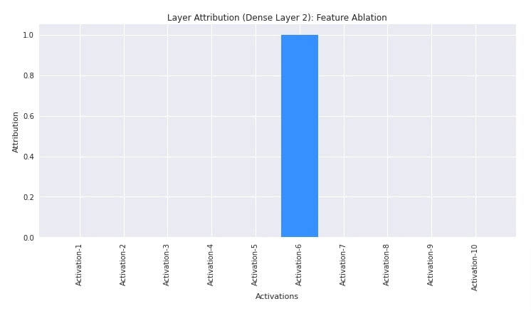
Layer Feature Ablation
In this section, we have explained the usage of layer feature ablation algorithm. We have created an algorithm using LayerFeatureAblation() constructor providing it our network and second linear layer. Then, we have generated activation contributions of the second layer towards the prediction of the first test example.
from captum import attr

interpreter = attr.LayerFeatureAblation(classifier, layers[1])
attributions = interpreter.attribute(X_test_classif[:1], target=Y_test_classif[:1])

attributions
import matplotlib.pyplot as plt
import matplotlib

with matplotlib.style.context("seaborn"):
    plt.figure(figsize=(12,5.5))
    plt.bar(range(10), attributions.mean(axis=0), width=0.85, color="dodgerblue");
    plt.xticks(range(10), ["Activation-{}".format(i+1) for i in range(10)], rotation=90)
    plt.xlabel("Activations");
    plt.ylabel("Attribution")
    plt.title("Layer Attribution (Dense Layer 2): Feature Ablation");
3. Neuron Attribution
In this section, we have explained the usage of algorithms from neuron attribution category. As explained earlier, the algorithm in this category let us find out the contributions of input data features towards the activation of a particular neuron of the selected layer.
Neuron Integrated Gradients
In this section, we have explained the usage of neuron integrated gradients algorithm. We have created an algorithm using NeuronIntegratedGradients() constructor. We have provided a classification network and a second linear layer to the constructor. Then, we have called attribute() method on the first test example. We have provided neuron_selector parameter with value 5 hinting that we want to find out the contributions of input data features towards the 6th neuron of the second linear layer. After deriving contributions, we have plotted them as well. We can find out from visualization features contributing positively and negatively toward the activation of a neuron.
layers = list(classifier.children())

layers
from captum import attr

interpreter = attr.NeuronIntegratedGradients(classifier, layers[1])
attributions = interpreter.attribute(X_test_classif[:1], neuron_selector=5)

attributions
import matplotlib.pyplot as plt
import matplotlib
with matplotlib.style.context("seaborn"):
plt.figure(figsize=(12,5.5))
plt.bar(range(n_features_classif), attributions.mean(axis=0), width=0.85, color="dodgerblue");
plt.xticks(range(n_features_classif), data_classif.feature_names, rotation=90)
plt.xlabel("Features");
plt.ylabel("Attribution")
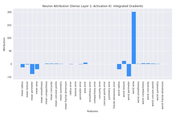
plt.title("Neuron Attribution (Dense Layer 2, Activation 6): Integrated Gradients");
Neuron Feature Ablation
In this section, we have explained the usage of neuron feature ablation. We have created algorithm using NeuronFeatureAblation() constructor. Then, we have generated contributions for the first test example using attribute() method. We have generated contributions of input features towards the activation of the 6th neuron of the second linear layer. After generating contributions, we have plotted them as well for reference purposes.
from captum import attr

interpreter = attr.NeuronFeatureAblation(classifier, layers[1])
attributions = interpreter.attribute(X_test_classif[:1], neuron_selector=5)

attributions
import matplotlib.pyplot as plt
import matplotlib
with matplotlib.style.context("seaborn"):
plt.figure(figsize=(12,5.5))
plt.bar(range(n_features_classif), attributions.mean(axis=0), width=0.85, color="dodgerblue");
plt.xticks(range(n_features_classif), data_classif.feature_names, rotation=90)
plt.xlabel("Features");
plt.ylabel("Attribution")
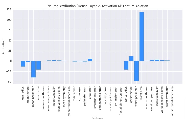
plt.title("Neuron Attribution (Dense Layer 2, Activation 6): Feature Ablation");
This ends our small tutorial explaining how we can interpret/explain predictions made by PyTorch networks using the Python captum library. Please feel free to let us know your views in the comments section.
References
Below, we have listed other Python libraries that can be used to explain predictions made by networks as well as visualize ML metrics.
- Captum: Interpret Predictions of PyTorch Image Classification Networks
- Captum: Explain Predictions of PyTorch Text Classification Networks
- How to Use LIME to Understand sklearn Models Predictions?
- How to Use eli5 to Understand sklearn Models, their Performance, and their Predictions?
- SHAP - Explain Machine Learning Model Predictions using Game Theoretic Approach
- Treeinterpreter - Interpreting Tree-Based Model's Prediction of Individual Sample
- Scikit-Plot: Visualizing Machine Learning Algorithm Results & Performance Metrics
- Yellowbrick - Visualize Sklearn's Classification & Regression Metrics in Python
- Yellowbrick - Text Data Visualizations
- interpret-text - Interpret NLP Models and Their Predictions
- dice-ml - Diverse Counterfactual Explanations for ML Models
- interpret-ml - Explain Machine Learning Models And Their Predictions
 Sunny Solanki
Sunny Solanki
Intro: Software Developer | Youtuber | Bonsai Enthusiast
About: Sunny Solanki holds a bachelor's degree in Information Technology (2006-2010) from L.D. College of Engineering. Post completion of his graduation, he has 8.5+ years of experience (2011-2019) in the IT Industry (TCS). His IT experience involves working on Python & Java Projects with US/Canada banking clients. Since 2020, he’s primarily concentrating on growing CoderzColumn.
His main areas of interest are AI, Machine Learning, Data Visualization, and Concurrent Programming. He has good hands-on with Python and its ecosystem libraries.
Apart from his tech life, he prefers reading biographies and autobiographies. And yes, he spends his leisure time taking care of his plants and a few pre-Bonsai trees.
Contact: sunny.2309@yahoo.in


![YouTube Subscribe]() Comfortable Learning through Video Tutorials?
Comfortable Learning through Video Tutorials?
If you are more comfortable learning through video tutorials then we would recommend that you subscribe to our YouTube channel.
![Need Help]() Stuck Somewhere? Need Help with Coding? Have Doubts About the Topic/Code?
Stuck Somewhere? Need Help with Coding? Have Doubts About the Topic/Code?
 Stuck Somewhere? Need Help with Coding? Have Doubts About the Topic/Code?
When going through coding examples, it's quite common to have doubts and errors.
If you have doubts about some code examples or are stuck somewhere when trying our code, send us an email at coderzcolumn07@gmail.com. We'll help you or point you in the direction where you can find a solution to your problem.
You can even send us a mail if you are trying something new and need guidance regarding coding. We'll try to respond as soon as possible.
![Share Views]() Want to Share Your Views? Have Any Suggestions?
Want to Share Your Views? Have Any Suggestions?
 Want to Share Your Views? Have Any Suggestions?
If you want to
- provide some suggestions on topic
- share your views
- include some details in tutorial
- suggest some new topics on which we should create tutorials/blogs
 captum, interpretation, pytorch-networks