Haiku (JAX): Word Embeddings for Text Classification Tasks
Nowadays, many of the NLP tasks (like text classification, text generation, sentiment analysis, etc) are getting solved by developing deep neural networks. Deep neural networks are complicated mathematical functions internally that work on real-valued data to solve given tasks. In order to make deep neural networks work for text data, we need some way to represent text data as real-valued data. There are many different approaches to encoding text data before giving it to neural networks. Famous approaches are word-frequency, one-hot, Tf-IDf, embeddings, etc. Approaches like word-frequency, one-hot, and tf-idf use only one real value to represent a single text token (word/character). This has limitations as the same word can be used in a different context and a single value can not capture all meanings. To solve it, embeddings were introduced which uses a real-valued vector to represent a word/character. As more values are getting used to represent a single word/character, it gives more representation power to it.
As a part of this tutorial, we have explained how to create neural networks using Python deep learning library Haiku that uses word embeddings approach to solving text classification tasks. Haiku is a high-level deep learning library designed on top of low-level library JAX. We have explained different ways of handling embeddings through our network to get better results. Each approach is evaluated by calculating various ML metrics. The predictions are analyzed further using LIME algorithm.
Below, we have listed essential tutorial sections to give an overview of the material covered.
Important Sections Of Tutorial
- Prepare Data
- 1.1 Load Data
- 1.2 Populate Vocabulary and Vectorize Data
- Approach 1: Flattened Embeddings
- 2.1 Define Network
- 2.2 Define Loss Function
- 2.3 Train Network
- 2.4 Evaluate Network Performance
- 2.5 Explain Network Predictions using LIME Algorithm
- Approach 2: Averaged Embeddings
- Approach 3: Summed Embeddings
- Summary of Results
- Further Suggestions
Below, we have imported the necessary Python libraries and printed the versions we used in our tutorial.
Haiku Installation
- !pip install -U dm-haiku
import haiku as hk

print("Haiku Version :{}".format(hk.__version__))
import jax

print("JAX Version : {}".format(jax.__version__))
import optax

print("Optax Version : {}".format(optax.__version__))
import torchtext

print("Torchtext Version : {}".format(torchtext.__version__))
1. Prepare Data 
In this section, we are preparing data for our neural network. We'll be following the below steps to prepare data for our network.
- Load Data.
- Tokenize each text example and Populate the vocabulary with unique words. A vocabulary is a simple mapping from a word to an integer index. Each word is assigned a unique index starting from 0.
- Vectorize text examples - Tokenize text examples and retrieve the index for each word from the vocabulary.
After performing the above 3 steps, we'll finally have an array of integer indexes where each index will be mapped to some word as per vocabulary.
The embedding will be implemented in a neural network as an embedding layer. This layer will have embeddings (a real-valued vector) for each word as a weight matrix. We'll retrieve embeddings for words by indexing this weight matrix using integer indexes that we retrieved from the vocabulary for each word. Don't worry if steps are not 100% clear to you as they'll become pretty clear once we implement them below.
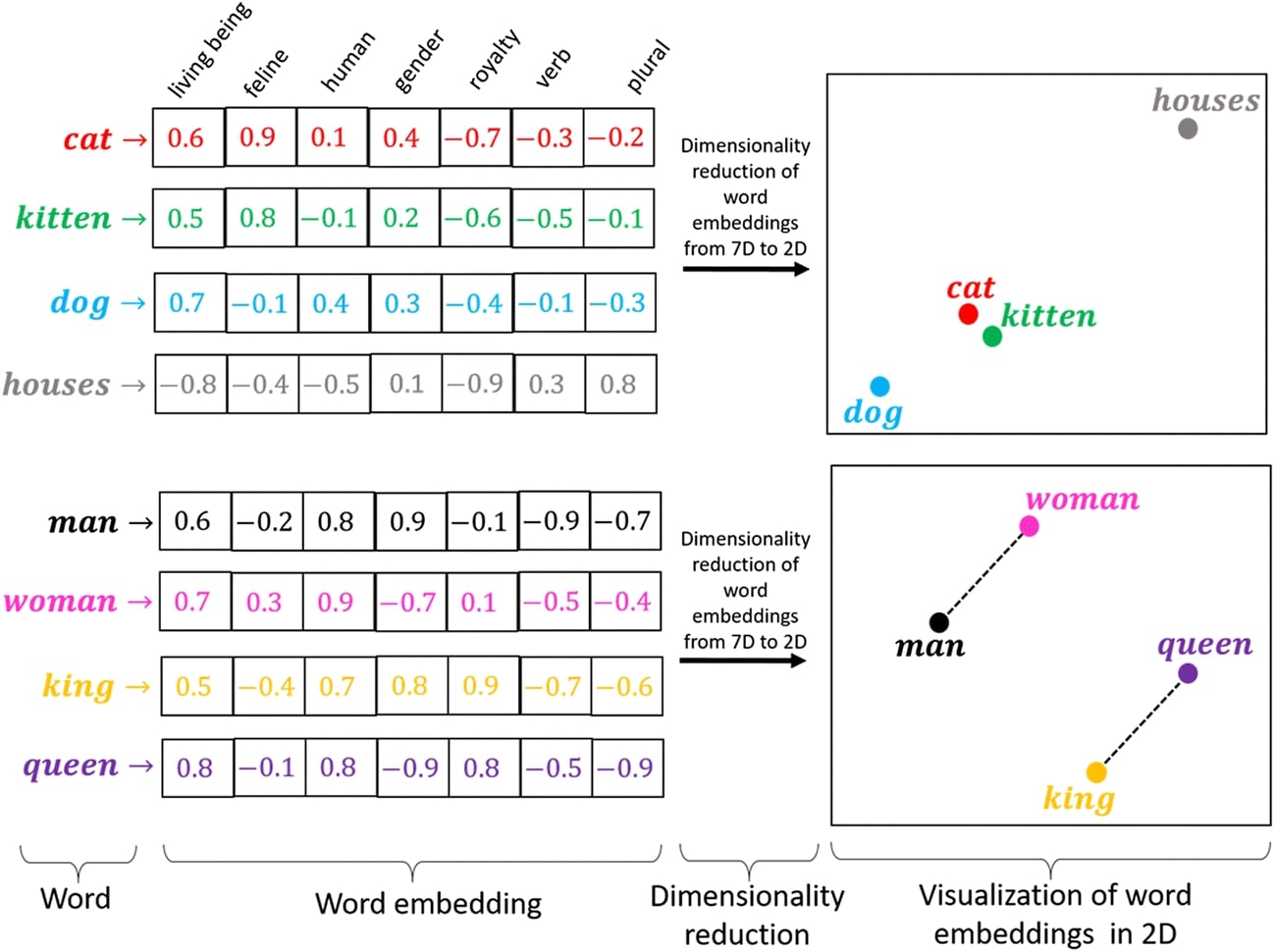
Below, we have included an image to give an idea about word embeddings.
1.1 Load Data
Below, we have loaded AG NEWS dataset available from torchtext python library. The dataset has news articles from 4 different news categories (["World", "Sports", "Business", "Sci/Tech"]). The dataset is already divided into train and test sets.
import numpy as np
import gc

train_dataset, test_dataset = torchtext.datasets.AG_NEWS()

X_train_text, Y_train = [], []
for Y, X in train_dataset:
    X_train_text.append(X)
    Y_train.append(Y)

X_test_text, Y_test = [], []
for Y, X in test_dataset:
    X_test_text.append(X)
    Y_test.append(Y)

unique_classes = list(set(Y_train))
target_classes = ["World", "Sports", "Business", "Sci/Tech"]

#Subtracted 1 from labels to bring range from 1-4 to 0-3
Y_train, Y_test = np.array(Y_train) - 1, np.array(Y_test) - 1

len(X_train_text), len(X_test_text)
1.2 Populate Vocabulary and Vectorize Data
Here, we are performing steps 2 (populate vocabulary) and 3 (vectorize data) that we had discussed earlier.
First, we have created an instance of Tokenizer which is available from the Python deep learning library Keras. It'll help us tokenize data, populate vocabulary and vectorize data as well.
After initializing the tokenizer object, we have populated vocabulary by calling fit_on_texts() method on it with train and test text examples. This method will loop through all text examples one by one, tokenize them, and populate vocabulary with unique words. Tokenization is a process where we break text into a list of tokens (words). We have also printed the size of vocabulary which is available through index_word and word_index attributes of the tokenizer object. We have also printed the first few mappings from the dictionary to show its contents.
As a next step, we have vectorized data where we tokenize text examples and retrieve their index from the vocabulary. We have performed this step by calling texts_to_sequences() method on the tokenizer object with train and test text examples one by one. The output of this step will be a list of integers for each text example where the integer will represent an index of the word as per vocabulary.
The size of the text example is different for each text example. But we need to prepare a dataset that has the same size for each example for the network. In order to do this, we have decided that we'll keep only the first 50 words from the text and will keep indexes of only them. We have completed this step using pad_sequences() method. This method makes sure that each example is of length 50. The examples that have more than 50 indexes will be truncated at 50 and examples that have less than 50 tokens will be padded with 0s.
After vectorizing datasets, we have converted them to JAX arrays as required by Haiku networks.
from keras.preprocessing.text import Tokenizer
from keras.preprocessing.sequence import pad_sequences
from jax import numpy as jnp

max_tokens = 50

tokenizer = Tokenizer()
tokenizer.fit_on_texts(X_train_text+X_test_text)

print("Vocabulary Size : {}".format(len(tokenizer.index_word)))

print("Vocabulary Starts @ Index 1: {}".format(list(tokenizer.index_word.items())[:5]))

X_train_vect = pad_sequences(tokenizer.texts_to_sequences(X_train_text), maxlen=max_tokens, padding="post", truncating="post", value=0.)
X_test_vect  = pad_sequences(tokenizer.texts_to_sequences(X_test_text), maxlen=max_tokens, padding="post", truncating="post", value=0.)

X_train_vect, X_test_vect = jnp.array(X_train_vect, dtype=jnp.int32), jnp.array(X_test_vect, dtype=jnp.int32)
Y_train, Y_test = jnp.array(Y_train), jnp.array(Y_test)

X_train_vect.shape, X_test_vect.shape
print(X_train_vect[:3])
# what is word 444

print(tokenizer.index_word[444])

## How many times it comes in first text document??
print()
print(X_train_text[0]) ## two times
2. Approach 1: Flattened Embeddings 
In this section, we have tried our first approach at using word embeddings. As we had discussed earlier, the embeddings for words will be present in the first layer of the network named Embedding layer. The embeddings for words will be retrieved by indexing them. The approach in this section flattens embeddings of single text example by stacking embeddings of words next to each other. These flattened embeddings are then given to dense layers for processing. Next, we'll check how this approach is performing on the dataset.
2.1 Define Network
Below, we have defined a network that we'll use for our text classification task. The network consists of 3 layers (One embedding and two linear).
The first layer of our network is the embedding layer. We have created an embedding layer using Embed() constructor available from haiku. We have given vocab size and embedding length to the constructor. The embedding length is set at 50 which means that each word index will have a real-valued vector of length 50. The constructor will internally create a weight matrix of shape (vocab_size, embed_len). As all of our examples are simple word indexes, the embedding for words will be retrieved by simply integer indexing this embedding matrix (E.g, let's say 'the' word has index 2, then embedding of 'the' will be 'weight_matrix[2]'). The input data shape to embedding layer is (batch_size, max_tokens) = (batch_size, 50) and output data shape is (batch_size, max_tokens, embed_len) = (batch_size, 50, 50).
The output of embedding layer is flattened as per our approach. This will transform shape from (batch_size, 50, 50) to (batch_size, 50 x 50) = (batch_size, 2500).
The flattened output will be given to our first linear layer which has 128 output units. The linear layer will process input data and will return the output of shape (batch_size, 128).
The output of the first linear layer is given to the second linear layer which has 4 output units (same as no of target classes). The output of the second linear layer is a prediction of our network.
After defining the network, we have transformed it to a pure JAX function (using hk.transform()) and initialized it. After initializing, we have printed the shape of weights/biases of layers of network and performed a forward pass through the network to make predictions for verification purposes.
If you are someone who is new to Haiku and want to learn how to create a neural network using it then we recommend that you go through our below tutorial. It'll get you started with haiku.
embed_len = 50

class EmbeddingClassifier(hk.Module):
    def __init__(self):
        super().__init__(name="EmbeddingClassifier")
        self.embedding = hk.Embed(vocab_size=len(tokenizer.word_index)+1, embed_dim=embed_len, name="Word_Embeddings")
        self.linear1 = hk.Linear(128, name="Dense1")
        self.linear2 = hk.Linear(len(target_classes), name="Dense2")
        self.flatten = hk.Flatten()

    def __call__(self, X_batch):
        x = self.embedding(X_batch) ## (batch_size, max_tokens, embed_len) = (1024, 50, 50)
        x = self.flatten(x) ## (batch_size, max_tokens x embed_len) = (32, 2500)
        x = self.linear1(x)
        return self.linear2(x)
def EmbeddingClassifierrNet(x):
    classif = EmbeddingClassifier()
    return classif(x)

embed_classif = hk.transform(EmbeddingClassifierrNet)
rng = jax.random.PRNGKey(42)

params = embed_classif.init(rng, X_train_vect[:5])

print("Weights Type : {}\n".format(type(params)))

for layer_name, weights in params.items():
    print(layer_name)
    #print(weights.keys())
    if "Embeddings" in layer_name:
        print("Embeddings : {}\n".format(weights["embeddings"].shape))
    else:
        print("Weights : {}, Biases : {}\n".format(params[layer_name]["w"].shape,params[layer_name]["b"].shape))
preds = embed_classif.apply(params, rng, X_train_vect[:5])

preds[:5]
2.2 Define Loss Function
In this section, we have defined a cross entropy loss function that we'll use for our classification task. The function takes network parameters, input data, and actual target labels as input. It then makes predictions using network parameters and input data. The actual target values are one-hot encoded. At last, loss is calculated by calling softmax_cross_entropy() function available from optax by giving predictions and one-hot encoded target values to it.
def CrossEntropyLoss(params, input_data, actual):
    logits_preds = model.apply(params, rng, input_data)
    one_hot_actual = jax.nn.one_hot(actual, num_classes=len(target_classes))
    return optax.softmax_cross_entropy(logits=logits_preds, labels=one_hot_actual).mean()
2.3 Train Network
In this section, we are training our network. To train the network, we have created a helper function. The function takes train data (X_train, Y_train), validation data (X_val, Y_val), number of epochs, network parameters, optimizer state, and batch size. The function executes a training loop number of epochs time. During each epoch, it loops through training data in batches. For each batch, it performs a forward pass to make predictions, calculates loss, calculates gradients, and updates network parameters. It records the loss of each batch and prints the average loss of all batches at the end of the epoch. It also calculates validation accuracy at the end of each epoch. At last, it returns updated network parameters.
from jax import value_and_grad
from tqdm import tqdm
from sklearn.metrics import accuracy_score

def TrainModelInBatches(X_train, Y_train, X_val, Y_val, epochs, params, optimizer_state, batch_size=32):
    for i in range(1, epochs+1):
        batches = jnp.arange((X_train.shape[0]//batch_size)+1) ### Batch Indices

        losses = [] ## Record loss of each batch
        for batch in tqdm(batches):
            if batch != batches[-1]:
                start, end = int(batch*batch_size), int(batch*batch_size+batch_size)
            else:
                start, end = int(batch*batch_size), None

            X_batch, Y_batch = X_train[start:end], Y_train[start:end] ## Single batch of data

            loss, gradients = value_and_grad(CrossEntropyLoss)(params, X_batch, Y_batch)

            #params = jax.tree_map(UpdateWeights, params, param_grads) ## Update Params
            updates, optimizer_state = optimizer.update(gradients, optimizer_state)
            params = optax.apply_updates(params, updates)
            losses.append(loss) ## Record Loss

        print("CrossEntropy Loss : {:.3f}".format(jnp.array(losses).mean()))
        gc.collect()
        Y_val_preds = model.apply(params, rng, X_val)
        val_acc = accuracy_score(Y_val, jnp.argmax(Y_val_preds, axis=1))
        print("Validation  Accuracy : {:.3f}".format(val_acc))
        gc.collect()
    return params
Below, we are actually training network by calling our training function defined in the previous cell. We have initialized a number of epochs to 12, batch size to 1024, and learning rate to 0.001. Then, we have initialized the model and Adam optimizer from optax. At last, we have called our training routine with necessary parameters to perform training process. We can notice from the loss and accuracy values getting printed at the end of each epoch that our network is doing a good job at the text classification task as loss is reducing and accuracy is increasing.
from jax import value_and_grad

rng = jax.random.PRNGKey(42) ## Reproducibility ## Initializes model with same weights each time.
epochs = 12
batch_size = 1024
learning_rate = 1e-3

model = hk.transform(EmbeddingClassifierrNet)
params = model.init(rng, X_train_vect[:5])
optimizer = optax.adam(learning_rate=learning_rate)
optimizer_state = optimizer.init(params)

final_params = TrainModelInBatches(X_train_vect, Y_train, X_test_vect, Y_test, epochs, params, optimizer_state, batch_size=batch_size)
2.4 Evaluate Network Performance
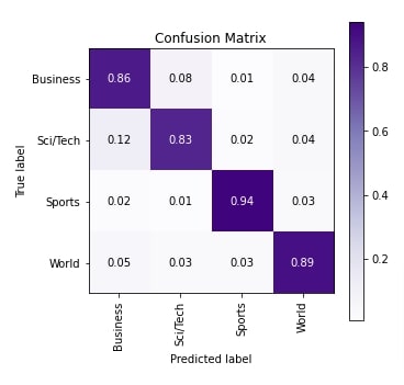
Below, we have evaluated the performance of our trained network by calculating metrics accuracy score, confusion matrix, and classification report (precision, recall, and f1-score) on the test dataset. We can notice from the accuracy score that our model is doing a good job at the given task. We have calculated these metrics using functions available from scikit-learn.
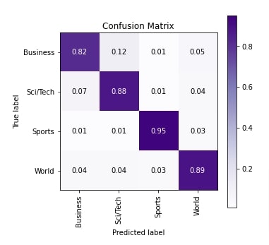
We have also created a heatmap of confusion matrix that let us see which categories are doing better compared to others. We can notice from the chart that categories 'Sports' and 'World' are doing better compared to categories 'Business' and 'Sci/Tech'.
We have created a chart using Python library scikit-plot. It has an implementation of charts for many different ML metrics. Please feel free to check the below link if you are new to the library and want to learn about it.
from sklearn.metrics import accuracy_score, classification_report, confusion_matrix

#train_preds = model.apply(final_params, rng, X_train_vect)
test_preds = model.apply(final_params, rng, X_test_vect)

#print("Train Accuracy : {:.3f}".format(accuracy_score(Y_train, np.argmax(train_preds, axis=1))))
print("Test  Accuracy : {:.3f}".format(accuracy_score(Y_test, np.argmax(test_preds, axis=1))))
print("\nClassification Report : ")
print(classification_report(Y_test, np.argmax(test_preds, axis=1), target_names=target_classes))
print("\nConfusion Matrix : ")
print(confusion_matrix(Y_test, np.argmax(test_preds, axis=1)))
from sklearn.metrics import confusion_matrix
import scikitplot as skplt
import matplotlib.pyplot as plt

skplt.metrics.plot_confusion_matrix([target_classes[i] for i in Y_test], [target_classes[i] for i in np.argmax(test_preds, axis=1)],
                                    normalize=True,
                                    title="Confusion Matrix",
                                    cmap="Purples",
                                    hide_zeros=True,
                                    figsize=(5,5)
                                    );
plt.xticks(rotation=90);
2.5 Explain Network Predictions using LIME Algorithm
In this section, we have dived deeper into checking the performance of our network. We are using LIME (Local Interpretable Model-Agnostic Explanations) algorithm to interpret prediction of the network which helps us understand which words of the network are contributing to the prediction. Thee is a python library named lime that provides an implementation of the algorithm. It let us create visualization which highlights words of text document that contributed to prediction.
If you are someone who is new to LIME then we would recommend that you go through the below link to understand it in-depth.
- How to Use LIME to Understand sklearn Models Predictions?
- LIME: Interpret Predictions Of Keras Text Classification Networks
In order to explain prediction using lime, we first need to create an instance of LimeTextExplainer which we have done below.
from lime import lime_text

explainer = lime_text.LimeTextExplainer(class_names=target_classes, verbose=True)
Below, we have created a prediction function. This function takes a list of text examples and returns predictions made by the network on them. It tokenizes and vectorizes them before giving them to the network. We'll use this function in the next cell for explaining predictions.
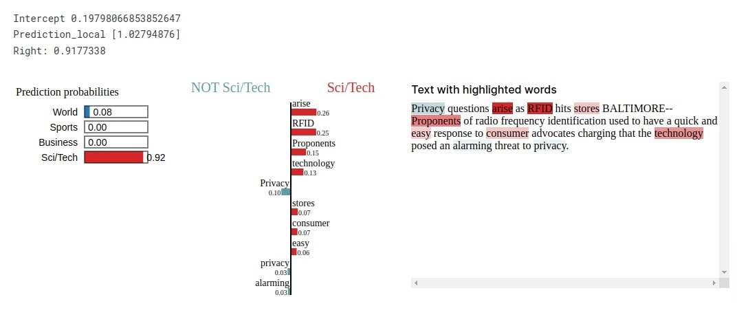
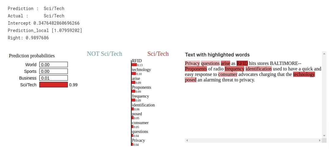
After defining a function, we randomly took a text example from the test dataset and made predictions on it using our trained network. Our network correctly predicts the target label as 'Sci/Tech' for the selected text example. Next, we'll look at which words of text document contributed to predicting this target category.
import numpy as np

def make_predictions(X_batch_text):
    X_batch = pad_sequences(tokenizer.texts_to_sequences(X_batch_text), maxlen=max_tokens, padding="post", truncating="post", value=0)
    preds = model.apply(final_params, rng, jnp.array(X_batch))
    preds = jax.nn.softmax(preds)
    return preds.to_py()

rnd_st = np.random.RandomState(1234)
idx = rnd_st.randint(1, len(X_test_text))

print("Prediction : ", target_classes[model.apply(final_params, rng, X_test_vect[idx:idx+1]).argmax(axis=-1)[0]])
print("Actual :     ", target_classes[Y_test[idx]])
Below, we have first created an Explanation object by calling explain_instance() method on the explainer object. We have provided a selected text example, prediction function, and actual target value to the function. The explanation object has details about words contributing to prediction.
Next, we have called show_in_notebook() method on the explanation object to create a visualization of the explanation. We can notice from the visualization that words like 'RFID', 'proponents', 'arise', 'technology', 'stores', 'consumer', etc are words contributing to predicting the target label as 'Sci/Tech' which makes sense as these are commonly used words in the tech industry. Though the network is still missing some important words which can contribute to prediction.
explanation = explainer.explain_instance(X_test_text[idx], classifier_fn=make_predictions, labels=Y_test[idx:idx+1].to_py())
explanation.show_in_notebook()
3. Approach 2: Averaged Embeddings 
In this section, we have explained another approach to using word embeddings. Our approach in this section takes embeddings of words of each text example and averages them before giving them to the linear layer. The only difference in architecture is that we are averaging embeddings at the text document level. The majority of the code in this section is the same as earlier.
3.1 Define Network
Below, we have defined the network that we'll use for our task. The network has the same number of layers as earlier with only a difference in forward pass. Here, we are taking the mean of embeddings before giving them to the linear layer instead of flattening them like earlier. The rest of the code is the same. We have initialized the network after defining it, printed shapes of weights/biases, and performed a forward pass for verification purposes.
embed_len = 50

class EmbeddingClassifier(hk.Module):
    def __init__(self):
        super().__init__(name="EmbeddingClassifier")
        self.embedding = hk.Embed(vocab_size=len(tokenizer.word_index)+1, embed_dim=embed_len, name="Word_Embeddings")
        self.linear1 = hk.Linear(128, name="Dense1")
        self.linear2 = hk.Linear(len(target_classes), name="Dense2")
        self.flatten = hk.Flatten()

    def __call__(self, X_batch):
        x = self.embedding(X_batch) ## (batch_size, max_tokens, embed_len) = (32, 50, 50)
        x = jnp.mean(x, axis=1) ## (batch_size, embed_len) = (32, 50)
        x = self.linear1(x)
        return self.linear2(x)
def EmbeddingClassifierrNet(x):
    classif = EmbeddingClassifier()
    return classif(x)

embed_classif = hk.transform(EmbeddingClassifierrNet)
rng = jax.random.PRNGKey(42)

params = embed_classif.init(rng, X_train_vect[:5])

print("Weights Type : {}\n".format(type(params)))

for layer_name, weights in params.items():
    print(layer_name)
    #print(weights.keys())
    if "Embeddings" in layer_name:
        print("Embeddings : {}\n".format(weights["embeddings"].shape))
    else:
        print("Weights : {}, Biases : {}\n".format(params[layer_name]["w"].shape,params[layer_name]["b"].shape))
preds = embed_classif.apply(params, rng, X_train_vect[:5])

preds[:5]
3.2 Train Network
Here, we have trained our new network architecture using the same settings that we had used earlier. We can notice from the loss and accuracy values that our network is doing a good job at the classification task.
from jax import value_and_grad

rng = jax.random.PRNGKey(42) ## Reproducibility ## Initializes model with same weights each time.
epochs = 12
batch_size = 1024
learning_rate = 1e-3

model = hk.transform(EmbeddingClassifierrNet)
params = model.init(rng, X_train_vect[:5])
optimizer = optax.adam(learning_rate=learning_rate)
optimizer_state = optimizer.init(params)

final_params = TrainModelInBatches(X_train_vect, Y_train, X_test_vect, Y_test, epochs, params, optimizer_state, batch_size=batch_size)
3.3 Evaluate Network Performance
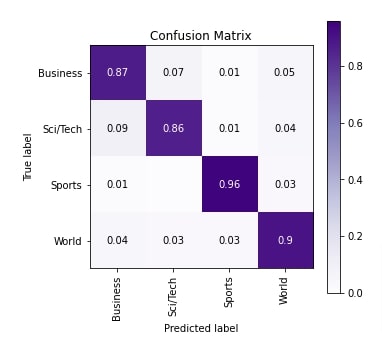
Below, we have evaluated the performance of our network as usual by calculating the accuracy score, confusion matrix, and classification report metrics on test predictions. We can clearly notice from the accuracy score that our model in this section is giving better results compared to the previous approach. We have also plotted the confusion matrix for reference purposes which hints at the improvement of all categories.
from sklearn.metrics import accuracy_score, classification_report, confusion_matrix

#train_preds = model.apply(final_params, rng, X_train_vect)
test_preds = model.apply(final_params, rng, X_test_vect)

#print("Train Accuracy : {:.3f}".format(accuracy_score(Y_train, np.argmax(train_preds, axis=1))))
print("Test  Accuracy : {:.3f}".format(accuracy_score(Y_test, np.argmax(test_preds, axis=1))))
print("\nClassification Report : ")
print(classification_report(Y_test, np.argmax(test_preds, axis=1), target_names=target_classes))
print("\nConfusion Matrix : ")
print(confusion_matrix(Y_test, np.argmax(test_preds, axis=1)))
from sklearn.metrics import confusion_matrix
import scikitplot as skplt
import matplotlib.pyplot as plt

skplt.metrics.plot_confusion_matrix([target_classes[i] for i in Y_test], [target_classes[i] for i in np.argmax(test_preds, axis=1)],
                                    normalize=True,
                                    title="Confusion Matrix",
                                    cmap="Purples",
                                    hide_zeros=True,
                                    figsize=(5,5)
                                    );
plt.xticks(rotation=90);
3.4 Explain Predictions using LIME Algorithm
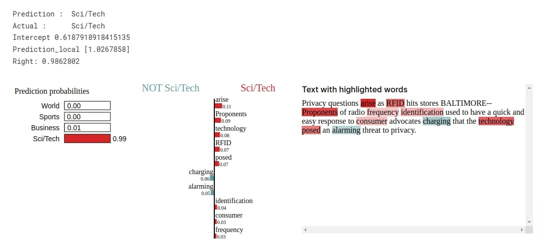
Here, we have explained network prediction using LIME algorithm. We have randomly selected text example and our model is correctly predicting target label as 'Sci/Tech' for it. The visualization shows that words like 'RFID', 'technology', 'arise', 'proponents', 'frequency', 'identification', 'consumer', 'questions', 'privacy', etc are contributing towards predicting target label as 'Sci/Tech'.
from lime import lime_text

explainer = lime_text.LimeTextExplainer(class_names=target_classes, verbose=True)

rnd_st = np.random.RandomState(1234)
idx = rnd_st.randint(1, len(X_test_text))

print("Prediction : ", target_classes[model.apply(final_params, rng, X_test_vect[idx:idx+1]).argmax(axis=-1)[0]])
print("Actual :     ", target_classes[Y_test[idx]])

explanation = explainer.explain_instance(X_test_text[idx], classifier_fn=make_predictions, labels=Y_test[idx:idx+1].to_py())
explanation.show_in_notebook()
4. Approach 3: Summed Embeddings 
In this section, we are trying a third way of using word embeddings for the text classification task. Our approach in this section is almost the same as our previous approach with the only change being that we are taking sum of embeddings at text document level instead of average. The rest of the code is exactly the same as earlier.
4.1 Define Network
Below, we have defined the network that we'll use for our task in this section. It has the same layers as our previous networks. The only difference is in forward pass where we are taking the sum of embeddings at the text document level before giving them to the linear layer. The rest of the logic is exactly the same. After defining the network, we initialized it, printed the shape of weights/biases, and performed a forward pass for verification.
embed_len = 50

class EmbeddingClassifier(hk.Module):
    def __init__(self):
        super().__init__(name="EmbeddingClassifier")
        self.embedding = hk.Embed(vocab_size=len(tokenizer.word_index)+1, embed_dim=embed_len, name="Word_Embeddings")
        self.linear1 = hk.Linear(128, name="Dense1")
        self.linear2 = hk.Linear(len(target_classes), name="Dense2")
        self.flatten = hk.Flatten()

    def __call__(self, X_batch):
        x = self.embedding(X_batch) ## (batch_size, max_tokens, embed_len) = (32, 50, 50)
        x = jnp.sum(x, axis=1) ## (batch_size, embed_len) = (32, 50)
        x = self.linear1(x)
        return self.linear2(x)
def EmbeddingClassifierrNet(x):
    classif = EmbeddingClassifier()
    return classif(x)

embed_classif = hk.transform(EmbeddingClassifierrNet)
rng = jax.random.PRNGKey(42)

params = embed_classif.init(rng, X_train_vect[:5])

print("Weights Type : {}\n".format(type(params)))

for layer_name, weights in params.items():
    print(layer_name)
    #print(weights.keys())
    if "Embeddings" in layer_name:
        print("Embeddings : {}\n".format(weights["embeddings"].shape))
    else:
        print("Weights : {}, Biases : {}\n".format(params[layer_name]["w"].shape,params[layer_name]["b"].shape))
preds = embed_classif.apply(params, rng, X_train_vect[:5])

preds[:5]
4.2 Train Network
Here, we have trained our network using the same settings that we have been using for all our previous approaches. We can notice from the loss and accuracy values that our network is doing a good job at the text classification task.
from jax import value_and_grad

rng = jax.random.PRNGKey(42) ## Reproducibility ## Initializes model with same weights each time.
epochs = 12
batch_size = 1024
learning_rate = 1e-3

model = hk.transform(EmbeddingClassifierrNet)
params = model.init(rng, X_train_vect[:5])
optimizer = optax.adam(learning_rate=learning_rate)
optimizer_state = optimizer.init(params)

final_params = TrainModelInBatches(X_train_vect, Y_train, X_test_vect, Y_test, epochs, params, optimizer_state, batch_size=batch_size)
4.3 Evaluate Network Performance
Below, we have evaluated the performance of our trained network by calculating accuracy score, classification report, and confusion matrix metrics on test predictions. We can notice from the accuracy score that it is better compared to our first approach but a little less compared to our previous approach (averaged embeddings). We have also plotted the confusion matrix for reference purposes.
from sklearn.metrics import accuracy_score, classification_report, confusion_matrix

#train_preds = model.apply(final_params, rng, X_train_vect)
test_preds = model.apply(final_params, rng, X_test_vect)

#print("Train Accuracy : {:.3f}".format(accuracy_score(Y_train, np.argmax(train_preds, axis=1))))
print("Test  Accuracy : {:.3f}".format(accuracy_score(Y_test, np.argmax(test_preds, axis=1))))
print("\nClassification Report : ")
print(classification_report(Y_test, np.argmax(test_preds, axis=1), target_names=target_classes))
print("\nConfusion Matrix : ")
print(confusion_matrix(Y_test, np.argmax(test_preds, axis=1)))
from sklearn.metrics import confusion_matrix
import scikitplot as skplt
import matplotlib.pyplot as plt

skplt.metrics.plot_confusion_matrix([target_classes[i] for i in Y_test], [target_classes[i] for i in np.argmax(test_preds, axis=1)],
                                    normalize=True,
                                    title="Confusion Matrix",
                                    cmap="Purples",
                                    hide_zeros=True,
                                    figsize=(5,5)
                                    );
plt.xticks(rotation=90);
4.4 Explain Predictions using LIME Algorithm
Below, we have checked the performance of our network using LIME algorithm. We randomly selected a text example from the test dataset and made predictions on it using our trained network. The network correctly predicts the target label as 'Sci/Tech'. Then, we created a visualization explaining the prediction of a network. We can notice from the visualization that words like 'arise', 'proponents', 'technology', 'RFID', 'identification', 'frequency', 'consumer', etc are contributing to predicting target label as 'Sci/Tech'.
from lime import lime_text

explainer = lime_text.LimeTextExplainer(class_names=target_classes, verbose=True)

rnd_st = np.random.RandomState(1234)
idx = rnd_st.randint(1, len(X_test_text))

print("Prediction : ", target_classes[model.apply(final_params, rng, X_test_vect[idx:idx+1]).argmax(axis=-1)[0]])
print("Actual :     ", target_classes[Y_test[idx]])

explanation = explainer.explain_instance(X_test_text[idx], classifier_fn=make_predictions, labels=Y_test[idx:idx+1].to_py())
explanation.show_in_notebook()
5. Summary of Results 
| Approach | Embedding Length | Test Accuracy |
|---|---|---|
| 1: Flattened Embeddings | 50 | 87.9% |
| 2: Averaged Embeddings | 50 | 89.9% |
| 3: Summed Embeddings | 50 | 88.4% |
6. Further Suggestions 
- Try training network for more epochs.
- Try different embedding lengths. We have tried embedding a length of 50.
- Try adding more dense layers.
- Try trained embeddings like GloVe, FastText, etc.
- Try other aggregation operations (max, min, etc) on embeddings. We tried averaging and summing.
- Try more max tokens per text example. We have kept only 50 tokens per text example.
- Try different activation functions (relu, tanh, etc).
- Try different weight initialization methods.
- Try regularization
- Try learning rate schedules
 Sunny Solanki
Sunny Solanki
Intro: Software Developer | Youtuber | Bonsai Enthusiast
About: Sunny Solanki holds a bachelor's degree in Information Technology (2006-2010) from L.D. College of Engineering. Post completion of his graduation, he has 8.5+ years of experience (2011-2019) in the IT Industry (TCS). His IT experience involves working on Python & Java Projects with US/Canada banking clients. Since 2020, he’s primarily concentrating on growing CoderzColumn.
His main areas of interest are AI, Machine Learning, Data Visualization, and Concurrent Programming. He has good hands-on with Python and its ecosystem libraries.
Apart from his tech life, he prefers reading biographies and autobiographies. And yes, he spends his leisure time taking care of his plants and a few pre-Bonsai trees.
Contact: sunny.2309@yahoo.in


![YouTube Subscribe]() Comfortable Learning through Video Tutorials?
Comfortable Learning through Video Tutorials?
If you are more comfortable learning through video tutorials then we would recommend that you subscribe to our YouTube channel.
![Need Help]() Stuck Somewhere? Need Help with Coding? Have Doubts About the Topic/Code?
Stuck Somewhere? Need Help with Coding? Have Doubts About the Topic/Code?
 Stuck Somewhere? Need Help with Coding? Have Doubts About the Topic/Code?
When going through coding examples, it's quite common to have doubts and errors.
If you have doubts about some code examples or are stuck somewhere when trying our code, send us an email at coderzcolumn07@gmail.com. We'll help you or point you in the direction where you can find a solution to your problem.
You can even send us a mail if you are trying something new and need guidance regarding coding. We'll try to respond as soon as possible.
![Share Views]() Want to Share Your Views? Have Any Suggestions?
Want to Share Your Views? Have Any Suggestions?
 Want to Share Your Views? Have Any Suggestions?
If you want to
- provide some suggestions on topic
- share your views
- include some details in tutorial
- suggest some new topics on which we should create tutorials/blogs
 haiku, jax, text-classification, word-embeddings