Learning Rate Schedules For JAX Networks
JAX is a deep learning research framework designed in Python by google research teams. It provides an API that we can use to build deep neural networks. JAX also provides an implementation of many optimizers like SGD, Adam, adamax, etc that are used to better handle gradients update of network parameters. SGD is commonly used optimizers where we set the initial learning rate for the training and it stays constant throughout the training process. The research has shown that the results of the model can be improved by annealing/decreasing the learning rate over time during the training process. We start with the initial learning rate and then we use some formula to decrease the learning rate after completion of batch/epoch. This process of annealing learning rate is generally referred to as learning rate scheduling or learning rate annealing.
As a part of this tutorial, we'll explain how we can use various learning rate schedules available from JAX. The optimizers and schedulers are available from optimizers sub-module of example_libraries sub-module of JAX. JAX has a high level-framework named Flax that simplifies the process of creating neural networks and it recommends using Optax library for optimizers and schedulers. If the reader is looking for Optax schedulers then please check the below link.
We have selected a Fashion MNIST dataset as a part of this tutorial and trained a simple CNN (Convolutional Neural Network) on it to explain various schedulers.
The tutorial assumes that the reader has a background in JAX and knows how to design a neural network using it. It also assumes that the reader has basic knowledge of how neural network works and is trained. If you want to refer to JAX and how to create a neural network using it then please check the below links.
- JAX - (Numpy + Automatic Gradients) on Accelerators (GPUs/TPUs)
- Guide to Create Neural Networks using High-level JAX API
Below, we have listed down important sections of the tutorial to give an overview of the material covered in it.
Important Sections Of Tutorial
- Load Data
- Define CNN
- Define Loss
- Train Network With Different Schedulers
Below, we have imported JAX and printed the version of it that we have used in this tutorial.
import jax

print("JAX Version : {}".format(jax.__version__))
Load Data 
In this section, we have loaded the Fashion MNIST dataset available from keras. It has grayscale images of shape (28,28) pixels for 10 different fashion items. The dataset is already divided into the train (60k images) and test (10k images) sets. After loading datasets, we have converted them to JAX arrays and then introduced one extra dimension at the end to mimic channel dimension for images as required by convolution layers. Below is a mapping from index to class names.
| Label | Description |
|---|---|
| 0 | T-shirt/top |
| 1 | Trouser |
| 2 | Pullover |
| 3 | Dress |
| 4 | Coat |
| 5 | Sandal |
| 6 | Shirt |
| 7 | Sneaker |
| 8 | Bag |
| 9 | Ankle boot |
from tensorflow import keras
from jax import numpy as jnp

(X_train, Y_train), (X_test, Y_test) = keras.datasets.fashion_mnist.load_data()

X_train, X_test, Y_train, Y_test = jnp.array(X_train, dtype=jnp.float32),\
                                   jnp.array(X_test, dtype=jnp.float32),\
                                   jnp.array(Y_train, dtype=jnp.float32),\
                                   jnp.array(Y_test, dtype=jnp.float32)

X_train, X_test = X_train.reshape(-1,28,28,1), X_test.reshape(-1,28,28,1)

X_train, X_test = X_train/255.0, X_test/255.0

classes =  jnp.unique(Y_train)

X_train.shape, X_test.shape, Y_train.shape, Y_test.shape
Define CNN 
In this section, we have defined the CNN that we have used in our tutorial for our multi-class classification problem. The network is simple enough to understand. It has 2 convolution layers and one dense layer. The convolution layers have filter sizes of 32 and 16 respectively. Both apply kernels of size (3,3) on input data to them. We have also applied relu (rectified linear unit) activation to the output of both layers. After applying relu to the output of the second convolution layer, we have flattened the output and directed it to the dense layer. The dense layer has a number of units same as a number of classification classes which is 10 (10 fashion items) in our case. To the output of the dense layer, we have applied softmax activation function which will convert outputs to probability in the range [0,1] such that 10 probabilities of the individual sample will sum to 1.
We have created a network using stax high-level API of JAX. If you want to know about it then please feel free to check our tutorial on it.
In the next cell after defining, we have also initialized the network and its parameters. We have also printed the shape of parameters of individual layers of the network for explanation purposes. We have also performed a forward pass through the network using a few samples to make predictions to verify that network is working as per our expectations.
from jax.example_libraries import stax

conv_init, conv_apply = stax.serial(
    stax.Conv(32,(3,3), padding="SAME"),
    stax.Relu,
    stax.Conv(16, (3,3), padding="SAME"),
    stax.Relu,

    stax.Flatten,
    stax.Dense(len(classes)),
    stax.Softmax
)
rng = jax.random.PRNGKey(123)

weights = conv_init(rng, (18,28,28,1))

weights = weights[1] ## Weights are actually stored in second element of two value tuple

for w in weights:
    if w:
        w, b = w
        print("Weights : {}, Biases : {}".format(w.shape, b.shape))
preds = conv_apply(weights, X_train[:5])

preds.shape
Define Loss 
In this section, we have defined a loss function that we have used during training. We have used cross entropy loss. The function takes as input network parameters, data features (X_batch), and actual target values (Y_batch). It then calculates loss based on predictions and actual target values.
def CrossEntropyLoss(weights, X_batch, Y_batch):
    preds = conv_apply(weights, X_batch)
    one_hot_actual = jax.nn.one_hot(Y_batch, num_classes=len(classes))
    log_preds = jnp.log(preds)
    return - jnp.sum(one_hot_actual * log_preds)
1. Constant Learning Rate 
In this section, we have trained our CNN with a constant learning rate. We can use results from this section to compare with other sections when we apply various schedulers to our training process.
We have designed a small function below that will perform our training process. It takes data features (X), target values (Y), validation data (X_val, Y_val), number of epochs, optimizer state, and batch size as input. It then loops the training number of epoch times. Each time, it goes through the whole data in batches, calculating loss and updating gradients. At the end of the epoch, it prints the loss of training data. We also calculate the loss of validation data and print it as well.
from jax import value_and_grad
from tqdm import tqdm
from sklearn.metrics import accuracy_score

def TrainModelInBatches(X, Y, X_val, Y_val, epochs, opt_state, batch_size=32):
    for i in range(1, epochs+1):
        batches = jnp.arange((X.shape[0]//batch_size)+1) ### Batch Indices

        losses = [] ## Record loss of each batch
        for batch in tqdm(batches):
            if batch != batches[-1]:
                start, end = int(batch*batch_size), int(batch*batch_size+batch_size)
            else:
                start, end = int(batch*batch_size), None

            X_batch, Y_batch = X[start:end], Y[start:end] ## Single batch of data

            loss, gradients = value_and_grad(CrossEntropyLoss)(opt_get_weights(opt_state), X_batch,Y_batch)

            ## Update Weights
            opt_state = opt_update(i, gradients, opt_state)

            losses.append(loss) ## Record Loss

        print("CrossEntropyLoss : {:.3f}".format(jnp.array(losses).mean()))

        Y_val_preds = conv_apply(opt_get_weights(opt_state), X_val)
        print("Validation Accuracy : {}".format(accuracy_score(Y_val, jnp.argmax(Y_val_preds, axis=1))))

    return opt_state
Below, we are actually training our CNN using the training function defined above. We have initialized the learning rate to 0.0001, a number of epochs to 10 and batch size 256. We have then initialized network weights and SGD optimizer. We have then called our training routine that trains the network and returns the final optimizer state that has final updated network weights.
from jax.example_libraries import optimizers

seed = jax.random.PRNGKey(123)
learning_rate = jnp.array(1/1e4)
epochs = 10
batch_size=256

weights = conv_init(rng, (batch_size,28,28,1))
weights = weights[1]


opt_init, opt_update, opt_get_weights = optimizers.sgd(learning_rate)
opt_state = opt_init(weights)

final_opt_state = TrainModelInBatches(X_train, Y_train, X_test, Y_test, epochs, opt_state, batch_size=batch_size)
2. Exponential Decay 
In this section, we have trained our CNN using SGD with exponential decay. We can create exponential decay using exponential_decay() function of optimizers sub-module of JAX. We then give this function response to SGD which will use to retrieve the learning rate at any step of training. We can inform the scheduler to update the learning rate after each epoch or after each batch (step). We have explained both scenarios in this section. Below are important parameters of the scheduler.
- step_size - Initial learning rate.
- decay_steps - Number of steps for which to decay learning rate.
- decay_rate - The float specifying decay rate.
JAX internally uses the below logic to find the learning rate at the end of each epoch/step.
def schedule(step_number):
    return initial_learning_rate * decay_rate ** (step_number / decay_steps)
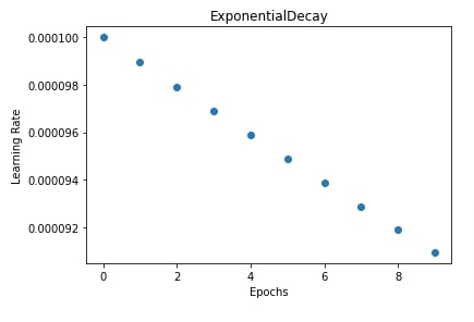
In our case, we have initialized exponential decay scheduler with an initial learning rate of 0.0001, steps the same as a number of epochs, and a decay rate of 0.9. We have then trained our network by giving this scheduler to SGD.
In the next cell after training, we have plotted a chart showing how the learning rate will change during training after each epoch.
seed = jax.random.PRNGKey(123)
learning_rate = jnp.array(1/1e4)
epochs = 10
batch_size=256

weights = conv_init(rng, (batch_size,28,28,1))
weights = weights[1]

exp_decay = optimizers.exponential_decay(0.0001, epochs, 0.9)
opt_init, opt_update, opt_get_weights = optimizers.sgd(exp_decay)
opt_state = opt_init(weights)

final_opt_state = TrainModelInBatches(X_train, Y_train, X_test, Y_test, epochs, opt_state, batch_size=batch_size)
import matplotlib.pyplot as plt

exp_decay = optimizers.exponential_decay(0.0001, epochs, 0.9)

lrs = [exp_decay(step) for step in range(epochs)]

plt.scatter(range(epochs), lrs);
plt.title("ExponentialDecay");
plt.xlabel("Epochs")
plt.ylabel("Learning Rate");
Below, we have redefined our training function which we had designed earlier. The only difference from the original training function is that number given to opt_update() function call is different here. Earlier, we had given a number that was the same as our epoch number. But this time, we are giving an actual number of the batch in the training process as input to opt_update() call. We are maintaining a separate counter named step for recording the count of each batch executed and we give this number to opt_update() call which will update the learning rate after each batch as opposed to the earlier call which was updated after each epoch.
from jax import value_and_grad
from tqdm import tqdm
from sklearn.metrics import accuracy_score

def TrainModelInBatches_Step(X, Y, X_val, Y_val, epochs, opt_state, batch_size=32):
    step=0
    for i in range(1, epochs+1):
        batches = jnp.arange((X.shape[0]//batch_size)+1) ### Batch Indices

        losses = [] ## Record loss of each batch
        for batch in tqdm(batches):
            if batch != batches[-1]:
                start, end = int(batch*batch_size), int(batch*batch_size+batch_size)
            else:
                start, end = int(batch*batch_size), None

            X_batch, Y_batch = X[start:end], Y[start:end] ## Single batch of data

            loss, gradients = value_and_grad(CrossEntropyLoss)(opt_get_weights(opt_state), X_batch,Y_batch)

            ## Update Weights
            opt_state = opt_update(step, gradients, opt_state)
            step += 1

            losses.append(loss) ## Record Loss

        print("CrossEntropyLoss : {:.3f}".format(jnp.array(losses).mean()))

        Y_val_preds = conv_apply(opt_get_weights(opt_state), X_val)
        print("Validation Accuracy : {}".format(accuracy_score(Y_val, jnp.argmax(Y_val_preds, axis=1))))

    return opt_state
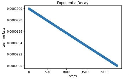
Below, we have trained our CNN with this new training function designed above which changes the learning rate after each batch/step using an exponential decay scheduler. We have also plotted how the learning rate will change during the training process now in the next cell.
seed = jax.random.PRNGKey(123)
learning_rate = jnp.array(1/1e4)
epochs = 10
batch_size=256
total_batches = (epochs*(X_train.shape[0]//batch_size)) + epochs

weights = conv_init(rng, (batch_size,28,28,1))
weights = weights[1]

exp_decay = optimizers.exponential_decay(0.0001, total_batches, 0.99)
opt_init, opt_update, opt_get_weights = optimizers.sgd(exp_decay)
opt_state = opt_init(weights)

final_opt_state = TrainModelInBatches_Step(X_train, Y_train, X_test, Y_test,epochs, opt_state, batch_size=batch_size)
import matplotlib.pyplot as plt

exp_decay = optimizers.exponential_decay(0.0001, total_batches, 0.99)

lrs = [exp_decay(step) for step in range(total_batches)]

plt.scatter(range(total_batches), lrs);
plt.title("ExponentialDecay");
plt.xlabel("Steps")
plt.ylabel("Learning Rate");
3. Inverse Time Decay 
In this section, we have trained our CNN using SGD with an inverse time decay scheduler. We can initialize inverse time decay scheduler using inverse_time_decay() function available from optimizers sub-module of JAX. Below are important parameters of the method.
- step_size - Initial learning rate.
- decay_steps - The number of steps for which to anneal learning rate.
- decay_rate - The rate at which anneal learning rate.
- staircase - It accepts boolean value specifying whether to decrease learning rate using staircase function.
Below logic is used internally by JAX to decide the learning rate using inverse time decay scheduler.
if staircase:
    def schedule(step_number):
        return initial_learning_rate / (1 + decay_rate * np.floor(step_number / decay_steps))
else:
    def schedule(step_number):
        return initial_learning_rate / (1 + decay_rate * step_number / decay_steps)
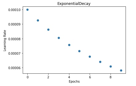
In our case, we have initialized inverse time decay scheduler with an initial learning rate of 0.0001, decay steps the same as a number of epochs, and decay rate of 0.8.
seed = jax.random.PRNGKey(123)
learning_rate = jnp.array(1/1e4)
epochs = 10
batch_size=256

weights = conv_init(rng, (batch_size,28,28,1))
weights = weights[1]

inv_time_decay = optimizers.inverse_time_decay(0.0001, 10, 0.8, staircase=True)
opt_init, opt_update, opt_get_weights = optimizers.sgd(inv_time_decay)
opt_state = opt_init(weights)

final_opt_state = TrainModelInBatches(X_train, Y_train, X_test, Y_test, epochs, opt_state, batch_size=batch_size)
import matplotlib.pyplot as plt

inv_time_decay = optimizers.inverse_time_decay(0.0001, epochs, 0.8, staircase=True)

lrs = [inv_time_decay(step) for step in range(epochs)]

plt.scatter(range(epochs), lrs);
plt.title("InverseTimeDecay");
plt.xlabel("Epochs")
plt.ylabel("Learning Rate");
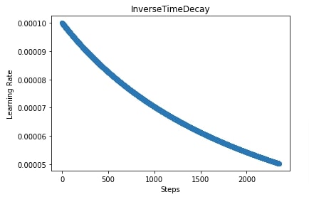
In the below cell, we are training our CNN again using SGD with inverse time decay scheduler but this time we have used a training function that anneals learning rate after each batch execution instead of after each epoch. We have also plotted learning rate changes during training in the next cell.
seed = jax.random.PRNGKey(123)
learning_rate = jnp.array(1/1e4)
epochs = 10
batch_size=256
total_batches = (epochs*(X_train.shape[0]//batch_size)) + epochs

weights = conv_init(rng, (batch_size,28,28,1))
weights = weights[1]

inv_time_decay = optimizers.inverse_time_decay(0.0001, total_batches, 0.99, staircase=True)
opt_init, opt_update, opt_get_weights = optimizers.sgd(inv_time_decay)
opt_state = opt_init(weights)

final_opt_state = TrainModelInBatches_Step(X_train, Y_train, X_test, Y_test, epochs, opt_state, batch_size=batch_size)
import matplotlib.pyplot as plt

inv_time_decay = optimizers.inverse_time_decay(0.0001, total_batches, 0.99, staircase=True)

lrs = [inv_time_decay(step) for step in range(total_batches)]

plt.scatter(range(total_batches), lrs);
plt.title("InverseTimeDecay");
plt.xlabel("Steps")
plt.ylabel("Learning Rate");
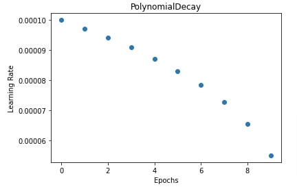
4. Polynomial Decay 
In this section, we have trained our CNN using SGD with a polynomial decay scheduler. We can create an inverse decay scheduler using polynomial_decay() function of optimizers sub-module. Below are important parameters of the function.
- step_size - Initial learning rate
- decay_steps - Total number of steps for which to anneal learning rate.
- final_step_size - Final learning rate after annealing.
- power - The power of polynomial formula for taking learning rate to final from initial.
Below is the logic internally used by JAX for the polynomial scheduler.
def schedule(step_number):
    step_number = np.minimum(step_number, decay_steps)
    step_mult = (1 - step_number / decay_steps) ** power
    return step_mult * (initial_learning_rate - final_learning_rate) + final_learning_rate
In our case, we have set the initial learning rate to 0.0001, the final learning rate to 0.00001, and power to 0.3.
In the next cell, we have also plotted how the learning rate will change during the training process. If we select a power value less than 1 then it'll create a concave curve and if we select it greater than 1 then it'll create the convex curve.
seed = jax.random.PRNGKey(123)
learning_rate = jnp.array(1/1e4)
epochs = 10
batch_size=256

weights = conv_init(rng, (batch_size,28,28,1))
weights = weights[1]

poly_decay = optimizers.polynomial_decay(0.0001, epochs, 0.00001, power=0.3)
opt_init, opt_update, opt_get_weights = optimizers.sgd(poly_decay)
opt_state = opt_init(weights)

final_opt_state = TrainModelInBatches(X_train, Y_train, X_test, Y_test, epochs, opt_state, batch_size=batch_size)
import matplotlib.pyplot as plt

poly_decay = optimizers.polynomial_decay(0.0001, epochs, 0.00001, power=0.3)

lrs = [poly_decay(step) for step in range(epochs)]

plt.scatter(range(epochs), lrs);
plt.title("PolynomialDecay");
plt.xlabel("Epochs")
plt.ylabel("Learning Rate");
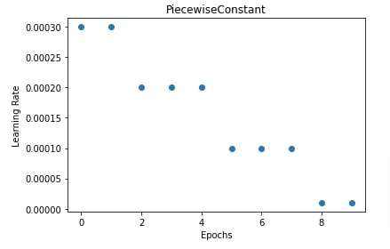
5. Piecewise Constant 
In this section, we have trained our CNN using SGD with the piecewise constant scheduler. We can create piecewise constant scheduler using piecewise_constant() function. It takes the below-mentioned parameters.
- boundaries - This parameter accepts a list of boundaries till which constant learning rates specified using values parameter will be used.
- values - This parameter accepts a list of learning rates and has a length one more than the boundaries parameter. It'll become clear below when explaining with examples how these parameters work.
Below is the internal logic of JAX for the piecewise constant scheduler.
def schedule(step_number):
    return values[np.sum(step_number > boundaries)]
In our case, we have initialized piecewise constant scheduler with boundaries set to [1,4,7] and learning rates to [0.0003, 0.0002, 0.0001, 0.00001]. This uses a learning rate of 0.0003 for 0th and 1st epochs, 0.0002 for 2nd, 3rd and 4th epochs, 0.0001 for 5th, 6th and 7th epochs, and 0.00001 for all epochs beyond the 7th epoch. The same logic can be applied when changing the learning rate after each batch.
seed = jax.random.PRNGKey(123)
learning_rate = jnp.array(1/1e4)
epochs = 10
batch_size=256

weights = conv_init(rng, (batch_size,28,28,1))
weights = weights[1]

piecewise_lr = optimizers.piecewise_constant([1,4,7], [0.0003, 0.0002, 0.0001, 0.00001])
opt_init, opt_update, opt_get_weights = optimizers.sgd(piecewise_lr)
opt_state = opt_init(weights)

final_opt_state = TrainModelInBatches(X_train, Y_train, X_test, Y_test, epochs, opt_state, batch_size=batch_size)
import matplotlib.pyplot as plt

piecewise_lr = optimizers.piecewise_constant([1,4,7], [0.0003, 0.0002, 0.0001, 0.00001])

lrs = [piecewise_lr(step) for step in range(epochs)]

plt.scatter(range(epochs), lrs);
plt.title("PiecewiseConstant");
plt.xlabel("Epochs")
plt.ylabel("Learning Rate");
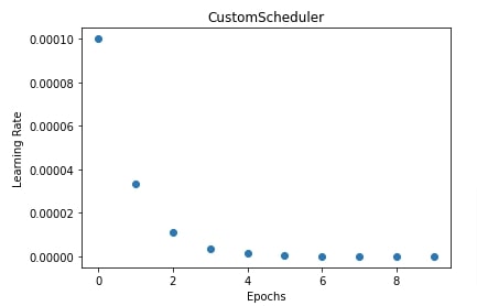
6. Custom Learning Rate Scheduler 
In this section, we have explained how we can create our own custom scheduler and use it if none of the existing schedulers is satisfying our requirements. In order to create a custom scheduler, we need to create a function that takes as input the parameters required for our scheduler. Then, we create one function inside of our main function that takes as input step number (epoch number/batch number) and returns the learning rate to use for that step number during training. The outer function returns an inner function which we can give to SGD which will use to retrieve the learning rate for a particular step number.
In our case, we have created a simple scheduler. The scheduler divides the learning rate by 3 at each step. We have then trained our CNN using SGD by providing this custom scheduler to it.
In the next cell, we have also explained how the learning rate will change during training if we use this scheduler.
def custom_scheduler(init_lr):
    def schedule(i):
        return init_lr if i==0 else init_lr / (3**i)
    return schedule
seed = jax.random.PRNGKey(123)
learning_rate = jnp.array(1/1e4)
epochs = 10
batch_size=256

weights = conv_init(rng, (batch_size,28,28,1))
weights = weights[1]

custom_scheduler = optimizers.make_schedule(custom_scheduler)
custom_lr = custom_scheduler(0.0001)
opt_init, opt_update, opt_get_weights = optimizers.sgd(custom_lr)
opt_state = opt_init(weights)

final_opt_state = TrainModelInBatches(X_train, Y_train, X_test, Y_test, epochs, opt_state, batch_size=batch_size)
import matplotlib.pyplot as plt

custom_scheduler = optimizers.make_schedule(custom_scheduler)
custom_lr = custom_scheduler(0.0001)

lrs = [custom_lr(step) for step in range(epochs)]

plt.scatter(range(epochs), lrs);
plt.title("CustomScheduler");
plt.xlabel("Epochs")
plt.ylabel("Learning Rate");
This ends our small tutorial explaining how we can use learning rate schedules for JAX networks. Please feel free to let us know your views in the comments section. The references section below includes other tutorials on the same or related topics. Please feel free to check them as well.
References
 Sunny Solanki
Sunny Solanki
Intro: Software Developer | Youtuber | Bonsai Enthusiast
About: Sunny Solanki holds a bachelor's degree in Information Technology (2006-2010) from L.D. College of Engineering. Post completion of his graduation, he has 8.5+ years of experience (2011-2019) in the IT Industry (TCS). His IT experience involves working on Python & Java Projects with US/Canada banking clients. Since 2020, he’s primarily concentrating on growing CoderzColumn.
His main areas of interest are AI, Machine Learning, Data Visualization, and Concurrent Programming. He has good hands-on with Python and its ecosystem libraries.
Apart from his tech life, he prefers reading biographies and autobiographies. And yes, he spends his leisure time taking care of his plants and a few pre-Bonsai trees.
Contact: sunny.2309@yahoo.in


![YouTube Subscribe]() Comfortable Learning through Video Tutorials?
Comfortable Learning through Video Tutorials?
If you are more comfortable learning through video tutorials then we would recommend that you subscribe to our YouTube channel.
![Need Help]() Stuck Somewhere? Need Help with Coding? Have Doubts About the Topic/Code?
Stuck Somewhere? Need Help with Coding? Have Doubts About the Topic/Code?
 Stuck Somewhere? Need Help with Coding? Have Doubts About the Topic/Code?
When going through coding examples, it's quite common to have doubts and errors.
If you have doubts about some code examples or are stuck somewhere when trying our code, send us an email at coderzcolumn07@gmail.com. We'll help you or point you in the direction where you can find a solution to your problem.
You can even send us a mail if you are trying something new and need guidance regarding coding. We'll try to respond as soon as possible.
![Share Views]() Want to Share Your Views? Have Any Suggestions?
Want to Share Your Views? Have Any Suggestions?
 Want to Share Your Views? Have Any Suggestions?
If you want to
- provide some suggestions on topic
- share your views
- include some details in tutorial
- suggest some new topics on which we should create tutorials/blogs
 jax, learning-rate-schedules