LIME: Explain Keras Image Classification Network (CNN) Predictions
LIME (Local Interpretable Model-Agnostic Explanations) is one of the most commonly used algorithms to explain the predictions of black-box models. We can generate feature importances when we are using ML models like linear regression, decision trees, random forests, gradient boosting trees, etc. But when we are using deep neural networks with many layers, it's hard to generate feature importances specifying how much each feature contributed to particular predictions. In those situations, LIME can help us. It internally generates a few fake samples from the input sample, trains a simple ML model (decision tree, linear regression, etc.) that can mimic the prediction of our black-box model (deep neural network), and use that simple model's prediction to explain the prediction of our black-box model. This helps us generate feature importances for our black-box model. We have a separate tutorial where we have covered how LIME works in detail. Please feel free to check it from the below link.
As a part of this tutorial, we'll be primarily concentrating on image classification tasks. We have created a keras convolution neural network and trained it on the Fashion MNIST dataset. Later on, we have used LIME to explain the predictions made by the model. We have plotted visualizations showing which parts of the images are contributing to prediction.
Below, we have listed important sections of our tutorial to give an overview of the material covered.
Important Sections Of Tutorial
- Load Data
- Create And Train Model
- Evaluate Network Performance
- Explain Predictions Using Lime Image Explainer
- 4.1 Explain True Prediction
- Pixels Contributing Positively to Prediction
- Pixels Contributing Negatively to Prediction
- 4.2 Explain True Predictions With Segmentation Method
- 4.3 Explain Wrong Prediction
- 4.1 Explain True Prediction
Below, we have imported the necessary libraries and printed the versions that we have used in our tutorial.
import tensorflow
from tensorflow import keras

print("Keras Version : {}".format(keras.__version__))
import lime

#print("LIME Version : {}".format(lime.__version__))
1. Load Data 
In this section, we have loaded the Fashion MNIST dataset available from keras. The dataset has grayscale images of shape (28,28) pixels of 10 different fashion items. The dataset is already divided into the train (60k images) and test (10k images) sets. Below, we have included a table that has a mapping from index to item names.
| Label | Description |
|---|---|
| 0 | T-shirt/top |
| 1 | Trouser |
| 2 | Pullover |
| 3 | Dress |
| 4 | Coat |
| 5 | Sandal |
| 6 | Shirt |
| 7 | Sneaker |
| 8 | Bag |
| 9 | Ankle boot |
from tensorflow import keras
from sklearn.model_selection import train_test_split
from jax import numpy as jnp
import numpy as np

(X_train, Y_train), (X_test, Y_test) = keras.datasets.fashion_mnist.load_data()

X_train, X_test = X_train.reshape(-1,28,28,1), X_test.reshape(-1,28,28,1)

X_train, X_test = X_train/255.0, X_test/255.0

classes =  np.unique(Y_train)
class_labels = ["T-shirt/top","Trouser","Pullover","Dress","Coat","Sandal","Shirt","Sneaker","Bag","Ankle boot"]
mapping = dict(zip(classes, class_labels))

X_train.shape, X_test.shape, Y_train.shape, Y_test.shape
2. Create And Train Model 
In this section, we have created a Convolution neural network for the image classification tasks and trained it. The network consists of 3 convolution layers and 1 dense layer. The three convolution layers have 48, 32, and 16 filters respectively with a kernel size of (3,3). All convolution layers have relu activation function. The output of the third convolution layer is flattened and given to the dense layer which has 10 units as input. The dense layer has softmax activation function.
After creating and initializing the network, we have compiled it to use Adam optimizer, cross entropy loss, and accuracy metric.
At last, we have trained the network for 10 epochs with a batch size of 256. We can notice from loss and accuracy getting printed after each epoch that the model is doing a good job at the image classification task.
from tensorflow.keras.models import Sequential
from tensorflow.keras import layers

model = Sequential([
    layers.Input(shape=X_train.shape[1:]),
    layers.Conv2D(filters=48, kernel_size=(3,3), padding="same", activation="relu"),
    layers.Conv2D(filters=32, kernel_size=(3,3), padding="same", activation="relu"),
    layers.Conv2D(filters=16, kernel_size=(3,3), padding="same", activation="relu"),

    layers.Flatten(),
    layers.Dense(len(classes), activation="softmax")
])

model.summary()
model.compile("adam", "sparse_categorical_crossentropy", ["accuracy"])
model.fit(X_train, Y_train, batch_size=256, epochs=10, validation_data=(X_test, Y_test))
3. Evaluate Network Performance 
In this section, we have evaluated the performance of the network by calculating accuracy, confusion matrix and classification report metrics on test predictions. We can notice from test accuracy that the model is doing a good job overall. When we look closely at the classification report and confusion matrix, we can notice that model is confused in categories T-shirt/top, Pullover, and Shirt. They have a little less accuracy compared to other categories.
We have used various functions available from scikit-learn to calculate various ML metrics. Please feel free to check the below link if you want to learn about them as the tutorial covers the majority of them.
from sklearn.metrics import accuracy_score, confusion_matrix, classification_report

Y_test_preds = model.predict(X_test)
Y_test_preds = np.argmax(Y_test_preds, axis=1)

print("Test Accuracy : {}".format(accuracy_score(Y_test, Y_test_preds)))
print("\nConfusion Matrix : ")
print(confusion_matrix(Y_test, Y_test_preds))
print("\nClassification Report :")
print(classification_report(Y_test, Y_test_preds, target_names=class_labels))
4. Explanation Using Lime Image Explainer 
In this section, we have explained predictions made by our model using an image explainer available from lime python library. In order to explain prediction using lime, we need to create an instance of LimeImageExplainer. Then, we can call explain_instance() method on it to create an instance of Explanation. The Explanation instance has details about pixels that contributed to prediction. We can call get_image_and_mask() method on Explanation instance to generate an image and a mask that can be plotted to see which pixels contributed to prediction.
Below, we have first created an instance of LimeImageExplainer using LimeImageExplainer() constructor available from lime_image sub-module of lime. We have not covered in detail various parameters of LimeImageExplainer() constructor here. Please feel free to check the below link if you want to tweak default settings.
from lime import lime_image
explainer = lime_image.LimeImageExplainer(random_state=123)

explainer
Create Prediction Function
In this section, we have created a simple function that takes images as input and makes predictions. This function will be required by explain_instance() method later. It simply returns 10 probabilities for each sample.
Please make a NOTE that our function takes as an input color image and works on it by converting it to a grayscale image. The reason behind this is that explain_instance() function of LimeImageExplainer can take the grayscale image as input but it converts the grayscale image to color before passing it to the prediction function.
import skimage
from skimage.color import gray2rgb, rgb2gray

def make_prediction(color_img):
    gray_img = rgb2gray(color_img).reshape(-1,28,28,1)
    preds = model.predict(gray_img)
    return preds
colored_image = gray2rgb(X_test[0].squeeze())

preds = make_prediction(colored_image)

preds.shape
4.1 Explain True Prediction 
In this section, we have explained the correct prediction made by our model. We have created separate visualizations showing pixels that contribute positively and negatively to prediction.
Below, we have first randomly selected a sample from test data. Then, we have printed the actual label of data and the predicted label. Then, we have called explain_instance() function with the test sample and prediction function. It generated an instance of Explanation which we'll use to generate an image and mask for visualization purposes next.
from skimage.segmentation import felzenszwalb, flood_fill, flood

rng = np.random.RandomState(42)
idx = rng.choice(range(len(X_test)))

print("Actual Target Value     : {}".format(mapping[Y_test[idx]]))
pred = model.predict(X_test[idx:idx+1]).argmax(axis=1)[0]
print("Predicted Target Values : {}".format(mapping[pred]))

explanation = explainer.explain_instance(X_test[idx].squeeze(), make_prediction, random_seed=123)

explanation
Pixels Contributing Positively to Prediction
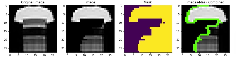
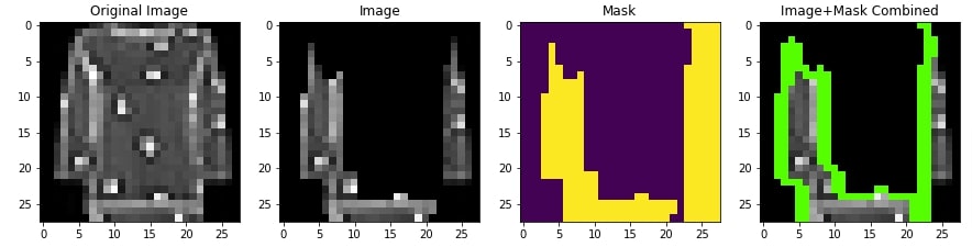
In this section, we have generated an image and mask that has pixels contributing positively to the prediction highlighted. We have given actual label as input to the get_image_and_mask() function of Explanation instance.
Then, in the next cell, we have displayed the actual image, the image returned by get_image_and_mask() function, mask, and combination of image and mask. This will help us compare and see which pixels contributed to the prediction. We can notice that the top and bottom pixels of the t-shirt are contributing to prediction positively.
img, mask = explanation.get_image_and_mask(Y_test[idx], positive_only=True, hide_rest=True)

img.shape, mask.shape
from skimage.segmentation import mark_boundaries
import matplotlib.pyplot as plt

def plot_comparison(main_image, img, mask):
    fig = plt.figure(figsize=(15,5))

    ax = fig.add_subplot(141)
    ax.imshow(main_image, cmap="gray");
    ax.set_title("Original Image")
    ax = fig.add_subplot(142)
    ax.imshow(img);
    ax.set_title("Image")
    ax = fig.add_subplot(143)
    ax.imshow(mask);
    ax.set_title("Mask")
    ax = fig.add_subplot(144)
    ax.imshow(mark_boundaries(img, mask, color=(0,1,0)));
    ax.set_title("Image+Mask Combined");

plot_comparison(X_test[idx], img, mask)
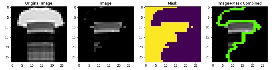
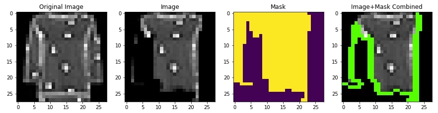
Pixels Contributing Negatively to Prediction
In this section, we have generated visualization showing pixels that contributes negatively to the prediction category. We have set negative_only parameter of method get_image_and_mask() function to True and positive_only parameter to False. We can notice from the visualization that some middle pixels are contributing negatively to prediction which means that they could be positively contributing to some other category.
img, mask = explanation.get_image_and_mask(Y_test[idx], positive_only=False, negative_only=True, hide_rest=True)

img.shape, mask.shape
plot_comparison(X_test[idx], img, mask)
4.2 Explain True Predictions With Segmentation Method 
In this section, we have again explained correct prediction but this time, we have provided different segmentation methods to explain_instance() function to see whether it makes any difference. We have used felzenszwalb segmentation method available from scikit-image library. We have generated a new explanation instance for a random test sample using felzenszwalb segmentation method.
from skimage.segmentation import felzenszwalb

rng = np.random.RandomState(42)
idx = rng.choice(range(len(X_test)))

print("Actual Target Value     : {}".format(mapping[Y_test[idx]]))
pred = model.predict(X_test[idx:idx+1]).argmax(axis=1)[0]
print("Predicted Target Values : {}".format(mapping[pred]))

explanation = explainer.explain_instance(X_test[idx].squeeze(), make_prediction,
                                         segmentation_fn=felzenszwalb, random_seed=123)

explanation
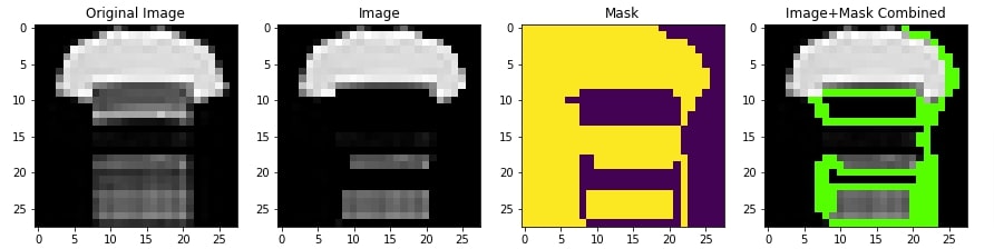
Pixels Contributing Positively to Prediction
In this section, we have created a visualization showing pixels contributing positively to the prediction category using an Explanation object created using felzenszwalb segmentation method.
img, mask = explanation.get_image_and_mask(Y_test[idx], positive_only=True, hide_rest=True)

plot_comparison(X_test[idx], img, mask)
Pixels Contributing Negatively to Prediction
In this section, we have created a visualization showing pixels contributing negatively to the prediction category using an Explanation object created using felzenszwalb segmentation method.
img, mask = explanation.get_image_and_mask(Y_test[idx], positive_only=False, negative_only=True, hide_rest=True)

plot_comparison(X_test[idx], img, mask)
4.3 Explain Wrong Prediction 
In this section, we have explained a wrong prediction made by our model. This will help us better understand which pixels are contributing to the prediction of the wrong category.
Below, we have first retrieved indexes of samples that are predicted wrong by our model. Then, we have randomly selected a sample that is predicted wrong by our model. The actual category of the selected sample is Pullover but our model predicts T-shirt/top. We have created an explanation instance as usual.
from skimage.segmentation import felzenszwalb

rng = np.random.RandomState(42)
idx = rng.choice(np.argwhere(Y_test!=Y_test_preds).flatten())

print("Actual Target Value     : {}".format(mapping[Y_test[idx]]))
pred = model.predict(X_test[idx:idx+1]).argmax(axis=1)[0]
print("Predicted Target Values : {}".format(mapping[pred]))

explanation = explainer.explain_instance(X_test[idx].squeeze(), make_prediction,
                                         segmentation_fn=felzenszwalb, random_seed=123)

explanation
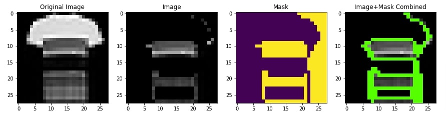
Pixels Contributing Positively to Prediction
In this section, we have created a visualization showing pixels that contribute positively to the actual category of the sample. We can notice from the results that it's missing important middle pixels that could have contributed to predicting the category Pullover.
img, mask = explanation.get_image_and_mask(Y_test[idx], positive_only=True, hide_rest=True)

plot_comparison(X_test[idx], img, mask)
Pixels Contributing Negatively to Prediction
In this section, we have created a visualization showing pixels that contribute negatively to predicting the actual category of the sample. We can notice that middle pixels which should have contributed positively to the prediction category are contributing negatively. This highlights that we need to work on our model and improve it further so that it can catch these kinds of patterns.
img, mask = explanation.get_image_and_mask(Y_test[idx], positive_only=False, negative_only=True, hide_rest=True)

plot_comparison(X_test[idx], img, mask)
This ends our small tutorial explaining how we can interpret the predictions made by the keras image classification network using LIME. Please feel free to let us know your views in the comments section.
References
 Sunny Solanki
Sunny Solanki
Intro: Software Developer | Youtuber | Bonsai Enthusiast
About: Sunny Solanki holds a bachelor's degree in Information Technology (2006-2010) from L.D. College of Engineering. Post completion of his graduation, he has 8.5+ years of experience (2011-2019) in the IT Industry (TCS). His IT experience involves working on Python & Java Projects with US/Canada banking clients. Since 2020, he’s primarily concentrating on growing CoderzColumn.
His main areas of interest are AI, Machine Learning, Data Visualization, and Concurrent Programming. He has good hands-on with Python and its ecosystem libraries.
Apart from his tech life, he prefers reading biographies and autobiographies. And yes, he spends his leisure time taking care of his plants and a few pre-Bonsai trees.
Contact: sunny.2309@yahoo.in


![YouTube Subscribe]() Comfortable Learning through Video Tutorials?
Comfortable Learning through Video Tutorials?
If you are more comfortable learning through video tutorials then we would recommend that you subscribe to our YouTube channel.
![Need Help]() Stuck Somewhere? Need Help with Coding? Have Doubts About the Topic/Code?
Stuck Somewhere? Need Help with Coding? Have Doubts About the Topic/Code?
 Stuck Somewhere? Need Help with Coding? Have Doubts About the Topic/Code?
When going through coding examples, it's quite common to have doubts and errors.
If you have doubts about some code examples or are stuck somewhere when trying our code, send us an email at coderzcolumn07@gmail.com. We'll help you or point you in the direction where you can find a solution to your problem.
You can even send us a mail if you are trying something new and need guidance regarding coding. We'll try to respond as soon as possible.
![Share Views]() Want to Share Your Views? Have Any Suggestions?
Want to Share Your Views? Have Any Suggestions?
 Want to Share Your Views? Have Any Suggestions?
If you want to
- provide some suggestions on topic
- share your views
- include some details in tutorial
- suggest some new topics on which we should create tutorials/blogs
 lime, image-classification, flax, JAX