MXNet: Learning Rate Schedules
When training neural networks, we generally keep the learning rate constant throughout the whole training process. But some research has shown that changing the learning rate over time can help improve the performance of the neural network. There are various formulas to decrease and increase learning rates in cycles over time to increase the accuracy of our network. This process of decreasing the learning rate over time during training is generally referred to as learning rate scheduling or learning rate annealing.
As a part of this tutorial, we have explained with examples how we can perform learning rate scheduling with mxnet networks. The mxnet many learning rate schedulers that we'll explore as a part of the tutorial. We have used the Fashion MNIST dataset for our purpose and trained a simple Convolutional Neural Network (CNN) on it. For training, we have used SGD optimizer with various learning rate schedulers from mxnet. We have also created various visualizations showing how the learning rate changes during training to give an idea about how the scheduler works. We assume that the reader has little background on mxnet. Please feel free to check the below links if you want to learn how to create CNN using mxnet.
Below, we have listed important sections of tutorial to give an overview of the material covered.
Important Sections Of Tutorial
- Load Data
- Define CNN
- Train Network Using Various Schedulers
Below, we have imported mxnet and printed the version that we have used in our tutorial.
import mxnet

print("MXNet Version : {}".format(mxnet.__version__))
Load Data 
Below, we have loaded the Fashion MNIST dataset which is available from keras. The dataset has grayscale images of shape (28,28) pixels for 10 different fashion items. The dataset is already divided into the train (60k images) and test (10k images) sets. After loading datasets, we have converted them from numpy arrays to mxnet arrays as required by mxnet networks. Below we have included a table that has a mapping from index to class names.
| Label | Description |
|---|---|
| 0 | T-shirt/top |
| 1 | Trouser |
| 2 | Pullover |
| 3 | Dress |
| 4 | Coat |
| 5 | Sandal |
| 6 | Shirt |
| 7 | Sneaker |
| 8 | Bag |
| 9 | Ankle boot |
from tensorflow import keras
from sklearn.model_selection import train_test_split

from mxnet import nd
import numpy as np

(X_train, Y_train), (X_test, Y_test) = keras.datasets.fashion_mnist.load_data()

X_train, X_test, Y_train, Y_test = nd.array(X_train, dtype=np.float32),\
                                   nd.array(X_test, dtype=np.float32),\
                                   nd.array(Y_train, dtype=np.float32),\
                                   nd.array(Y_test, dtype=np.float32)

X_train, X_test = X_train.reshape(-1,1,28,28), X_test.reshape(-1,1,28,28)

X_train, X_test = X_train/255.0, X_test/255.0

classes =  np.unique(Y_train.asnumpy())
class_labels = ["T-shirt/top","Trouser","Pullover","Dress","Coat","Sandal","Shirt","Sneaker","Bag","Ankle boot"]
mapping = dict(zip(classes, class_labels))

X_train.shape, X_test.shape, Y_train.shape, Y_test.shape
Define CNN 
In this section, we have defined a convolutional neural network that we'll use to classify images. The network has 2 convolution layers and one dense layer. The two convolution layers have 32 and 16 output channels respectively and both have a kernel of shape (3,3). Both convolution layers apply relu activation function to the output. The output of the second convolution layer is flattened and given to the dense layer as input. The dense layer has 10 output units (same as the target classes).
After defining the network, we have initialized it and made predictions using it for verification purposes.
from mxnet.gluon import nn

class CNN(nn.Block):
    def __init__(self, **kwargs):
        super(CNN, self).__init__(**kwargs)
        self.conv1 = nn.Conv2D(channels=32, kernel_size=(3,3), activation="relu", padding=(1,1))
        self.conv2 = nn.Conv2D(channels=16, kernel_size=(3,3), activation="relu", padding=(1,1))
        self.flatten = nn.Flatten()
        self.linear = nn.Dense(len(classes))

    def forward(self, x):
        x = self.conv1(x)
        x = self.conv2(x)

        x = self.flatten(x)
        logits = self.linear(x)
        return logits #nd.softmax(logits)

model = CNN()

model
from mxnet import init, initializer

model.initialize(initializer.Xavier())

preds = model(X_train[:5])

preds.shape
1. Constant Learning Rate 
In this section, we have trained our network using a constant learning rate. Below, we have created a function that we'll use throughout our tutorial for the training network. The function takes trainer object, training data (X, Y), validation data (X_val, Y_val), number of epochs, and batch size as input. It then performs a training loop number of epochs times. For each epoch, it loops through whole training data in batches. For each batch, it performs a forward pass to make predictions, calculate loss, calculate gradients, and update network parameters. We accumulate training loss for each batch and then print the average training loss at the end of each epoch. We also calculate validation loss at the end of each epoch and print it.
from mxnet import autograd
from tqdm import tqdm

def TrainModelInBatches(trainer, X, Y, X_val, Y_val, epochs, batch_size=32):
    for i in range(1, epochs+1):
        batches = nd.arange((X.shape[0]//batch_size)+1) ### Batch Indices

        losses = [] ## Record loss of each batch
        for batch in tqdm(batches):
            batch = batch.asscalar()
            if batch != batches[-1]:
                start, end = int(batch*batch_size), int(batch*batch_size+batch_size)
            else:
                start, end = int(batch*batch_size), None

            X_batch, Y_batch = X[start:end], Y[start:end] ## Single batch of data

            with autograd.record():
                preds = model(X_batch) ## Forward pass to make predictions
                train_loss = loss_func(preds.squeeze(), Y_batch) ## Calculate Loss
            train_loss.backward() ## Calculate Gradients

            train_loss = train_loss.mean().asscalar()
            losses.append(train_loss)

            trainer.step(len(X_batch)) ## Update weights

        print("Train CrossEntropyLoss : {:.3f}".format(np.array(losses).mean()))
        val_loss = loss_func(model(X_val), Y_val)
        print("Valid CrossEntropyLoss : {:.3f}".format(val_loss.mean().asscalar()))
In the below cell, we are training our network using a function defined in the previous cell. We have first initialized batch size to 256, a number of epochs to 25, and learning rate to 0.001. Then, we have initialized the network, loss function, optimizer, and trainer object. At last, we have called our training function to perform training. We can notice from the loss values getting printed after each epoch that our model is doing a good job.
from mxnet import gluon
from mxnet.gluon import loss
from mxnet import autograd
from mxnet import optimizer

batch_size=256
epochs=25
learning_rate = 0.001

model = CNN()
model.initialize()
loss_func = loss.SoftmaxCrossEntropyLoss()
grad_descent = optimizer.SGD(learning_rate=learning_rate)

trainer = gluon.Trainer(model.collect_params(), grad_descent)

TrainModelInBatches(trainer, X_train, Y_train, X_test, Y_test, epochs, batch_size=batch_size)
Below, we have made predictions on test data using our trained model. Then, we have calculated accuracy and a classification report on test predictions.
Below we have calculated metrics using functions available from scikit-learn. Please feel free to check the below link if you want to learn about various ML metrics available from scikit-learn.
from sklearn.metrics import accuracy_score, confusion_matrix, classification_report

Y_test_preds = model(X_test)
Y_test_preds = Y_test_preds.argmax(axis=-1)

print("Test Accuracy : {}".format(accuracy_score(Y_test_preds.asnumpy(), Y_test.asnumpy())))
print("Classification Report : ")
print(classification_report(Y_test_preds.asnumpy(), Y_test.asnumpy(), target_names=class_labels))
2. Factor Scheduler 
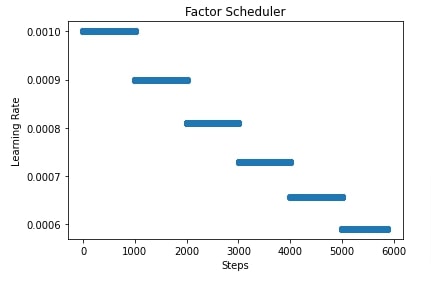
In this section, we have trained our network using SGD with a factor learning rate scheduler. It multiplies the current learning rate by a particular factor after a specified number of steps has passed to generate a new learning rate. We can create factor scheduler using FactorScheduler() constructor available from lr_scheduler sub-module of mxnet. Below are important parameters of the constructor.
- step - This parameter accepts integer specifying after how many steps (batches) to anneal learning rate.
- factor - This parameter accepts float value that is used to multiply the current learning rate after specified steps have passed to generate a new learning rate.
- base_lr - This is the initial learning rate.
- stop_factor_lr - This the minimum learning rate. The learning rate won't be decreased below this value.
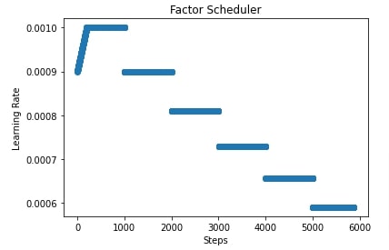
- warmup_steps - This parameter accepts integer value specifying the number of warm-up steps used by the scheduler before it starts annealing the learning rate.
- warmup_begin_lr - This parameter accepts the initial learning rate for warm-up steps. During warm-up steps learning rate starts with this learning rate and reaches till base learning rate.
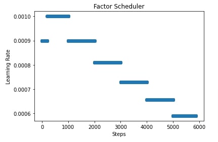
- warmup_mode - This parameter accepts string value specifying how the learning rate changes during warm-up steps.
- 'linear' - This will steadily increase the learning rate from warm-up LR to base LR.
- 'constant' - This will keep the learning rate constant at warm-up LR throughout warm-up steps.
The scheduler uses the below formula to anneal the learning rate.
base_lr * pow(factor, floor(num_update/step))In our case, we have initialized FactorScheduler with an initial learning rate of 0.001, steps after which to anneal learning rate to 1000, factor to 0.9, and minimum LR to 1e-6. This will start with an initial learning rate of 0.001 and multiply it by 0.9 after 1000 steps.
from mxnet import gluon
from mxnet.gluon import loss
from mxnet import autograd
from mxnet import optimizer
from mxnet import lr_scheduler

batch_size=256
epochs=25
learning_rate = 0.001

model = CNN()
model.initialize()
loss_func = loss.SoftmaxCrossEntropyLoss()

steps = (X_train.shape[0]//batch_size)*epochs + epochs
scheduler = lr_scheduler.FactorScheduler(step=1000, factor=0.9, stop_factor_lr=1e-6,
                                         base_lr=learning_rate)
grad_descent = optimizer.SGD(lr_scheduler=scheduler)

trainer = gluon.Trainer(model.collect_params(), grad_descent)

TrainModelInBatches(trainer, X_train, Y_train, X_test, Y_test, epochs, batch_size=batch_size)
In this cell, we have evaluated the performance of the network by calculating accuracy and classification report.
from sklearn.metrics import accuracy_score, confusion_matrix, classification_report

Y_test_preds = model(X_test)
Y_test_preds = Y_test_preds.argmax(axis=-1)

print("Test Accuracy : {}".format(accuracy_score(Y_test_preds.asnumpy(), Y_test.asnumpy())))
print("Classification Report : ")
print(classification_report(Y_test_preds.asnumpy(), Y_test.asnumpy(), target_names=class_labels))
In the next few cells, we have plotted how the learning rate will change during training if we use FactorScheduler with different settings. This helps us better understand how it works internally.
import matplotlib.pyplot as plt

scheduler = lr_scheduler.FactorScheduler(step=1000, factor=0.9,
                                         stop_factor_lr=1e-6, base_lr=learning_rate)

lrs = [scheduler(i) for i in range(steps)]
plt.scatter(range(steps), lrs)
plt.title('Factor Scheduler')
plt.xlabel("Steps")
plt.ylabel("Learning Rate");
import matplotlib.pyplot as plt

scheduler = lr_scheduler.FactorScheduler(step=1000, factor=0.9, stop_factor_lr=1e-6,
                                         base_lr=learning_rate, warmup_steps=200,
                                         warmup_begin_lr=0.0009)

lrs = [scheduler(i) for i in range(steps)]
plt.scatter(range(steps), lrs)
plt.title('Factor Scheduler')
plt.xlabel("Steps")
plt.ylabel("Learning Rate");
import matplotlib.pyplot as plt

scheduler = lr_scheduler.FactorScheduler(step=1000, factor=0.9, stop_factor_lr=1e-6,
                                         base_lr=learning_rate, warmup_steps=200,
                                         warmup_begin_lr=0.0009, warmup_mode="constant")

lrs = [scheduler(i) for i in range(steps)]
plt.scatter(range(steps), lrs)
plt.title('Factor Scheduler')
plt.xlabel("Steps")
plt.ylabel("Learning Rate");
3. Multi Factor Scheduler 
In this section, we have trained our network using SGD with a multi-factor learning rate scheduler. We can create multi-factor scheduler using MultiFactorScheduler() constructor. Below are important parameters of the constructor.
- step - This parameter accepts a list of integers specifying boundaries after which to modify the learning rate.
- factor - This parameter accepts float value that is used to multiply the current learning rate after specified steps have passed to generate a new learning rate.
- base_lr - This is the initial learning rate.
- warmup_steps - This parameter accepts integer value specifying the number of warm-up steps used by the scheduler before it starts annealing the learning rate.
- warmup_begin_lr - This parameter accepts the initial learning rate for warm-up steps. During warm-up steps learning rate starts with this learning rate and reaches till base learning rate.
- warmup_mode - This parameter accepts string value specifying how the learning rate changes during warm-up steps.
- 'linear' - This will steadily increase the learning rate from warm-up LR to base LR.
- 'constant' - This will keep the learning rate constant at warm-up LR throughout warm-up steps.
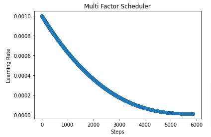
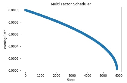
In our case, we have initialized MultiFactorScheduler() with step parameter set to [1000,2000,3000], factor parameter set to 0.9 and base LR set to 0.001. This will keep the learning rate at 0.001 for the first 1000 steps, then it'll multiply the learning rate by 0.9 for the next 1000 steps. Then, it'll again multiply the learning rate by 0.9 for the next 1000 steps. Then, it'll again multiply the learning rate by 0.9 for all steps beyond 3000 steps.
In the next cell, we have also evaluated the performance of the network by calculating accuracy and classification report metrics.
In the cell after metrics calculation, we have also plotted how the learning rate will change during training if we use a multi-factor scheduler to anneal it.
from mxnet import gluon
from mxnet.gluon import loss
from mxnet import autograd
from mxnet import optimizer
from mxnet import lr_scheduler

batch_size=256
epochs=25
learning_rate = 0.001

model = CNN()
model.initialize()
loss_func = loss.SoftmaxCrossEntropyLoss()

steps = (X_train.shape[0]//batch_size)*epochs + epochs
scheduler = lr_scheduler.MultiFactorScheduler(step=[1000,2000,3000], factor=0.9, base_lr=learning_rate)
grad_descent = optimizer.SGD(lr_scheduler=scheduler)

trainer = gluon.Trainer(model.collect_params(), grad_descent)

TrainModelInBatches(trainer, X_train, Y_train, X_test, Y_test, epochs, batch_size=batch_size)
from sklearn.metrics import accuracy_score, confusion_matrix, classification_report

Y_test_preds = model(X_test)
Y_test_preds = Y_test_preds.argmax(axis=-1)

print("Test Accuracy : {}".format(accuracy_score(Y_test_preds.asnumpy(), Y_test.asnumpy())))
print("Classification Report : ")
print(classification_report(Y_test_preds.asnumpy(), Y_test.asnumpy(), target_names=class_labels))
import matplotlib.pyplot as plt

scheduler = lr_scheduler.MultiFactorScheduler(step=[1000,2000,3000], factor=0.9, base_lr=learning_rate)

lrs = [scheduler(i) for i in range(steps)]
plt.scatter(range(steps), lrs)
plt.title('Multi Factor Scheduler')
plt.xlabel("Steps")
plt.ylabel("Learning Rate");

4. Polynomial Scheduler 
In this section, we have trained our network using SGD with the polynomial scheduler. We can create polynomial scheduler using PolyScheduler() constructor available from lr_scheduler sub-module. Below are important parameters of the scheduler.
- max_update - This parameter accepts integer specifying number of steps for which to anneal learning rate.
- base_lr - This is the initial learning rate.
- pwr - This parameter accepts integers specifying the power of the decay term.
- final_lr - This is the final learning rate after max_update steps are completed.
- warmup_steps - This parameter accepts integer value specifying the number of warm-up steps used by the scheduler before it starts annealing the learning rate.
- warmup_begin_lr - This parameter accepts the initial learning rate for warm-up steps. During warm-up steps learning rate starts with this learning rate and reaches till base learning rate.
- warmup_mode - This parameter accepts string value specifying how the learning rate changes during warm-up steps.
- 'linear' - This will steadily increase the learning rate from warm-up LR to base LR.
- 'constant' - This will keep the learning rate constant at warm-up LR throughout warm-up steps.
In our case, we have created a polynomial scheduler with max_update set to total training batches, power set to 2.5, base learning rate set to 0.001, and final learning rate set to 1e-5. After training the network, we have also evaluated accuracy and classification report on test predictions.
In the cells after accuracy calculation, we have plotted a chart showing how the learning rate will change during training if we use a polynomial scheduler with different settings. If we keep power greater than 1 then the shape of the line in the chart will be convex else it'll be concave if power is less than 1.
from mxnet import gluon
from mxnet.gluon import loss
from mxnet import autograd
from mxnet import optimizer
from mxnet import lr_scheduler

batch_size=256
epochs=25
learning_rate = 0.001

model = CNN()
model.initialize()
loss_func = loss.SoftmaxCrossEntropyLoss()

steps = (X_train.shape[0]//batch_size)*epochs + epochs
scheduler = lr_scheduler.PolyScheduler(max_update=steps, pwr=2.5, base_lr=learning_rate, final_lr=1e-5)
grad_descent = optimizer.SGD(lr_scheduler=scheduler)

trainer = gluon.Trainer(model.collect_params(), grad_descent)

TrainModelInBatches(trainer, X_train, Y_train, X_test, Y_test, epochs, batch_size=batch_size)
from sklearn.metrics import accuracy_score, confusion_matrix, classification_report

Y_test_preds = model(X_test)
Y_test_preds = Y_test_preds.argmax(axis=-1)

print("Test Accuracy : {}".format(accuracy_score(Y_test_preds.asnumpy(), Y_test.asnumpy())))
print("Classification Report : ")
print(classification_report(Y_test_preds.asnumpy(), Y_test.asnumpy(), target_names=class_labels))
import matplotlib.pyplot as plt

scheduler = lr_scheduler.PolyScheduler(max_update=steps, pwr=2.5, base_lr=learning_rate, final_lr=1e-5)

lrs = [scheduler(i) for i in range(steps)]
plt.scatter(range(steps), lrs)
plt.title('Multi Factor Scheduler')
plt.xlabel("Steps")
plt.ylabel("Learning Rate");
import matplotlib.pyplot as plt

scheduler = lr_scheduler.PolyScheduler(max_update=steps, pwr=0.5, base_lr=learning_rate, final_lr=1e-5)

lrs = [scheduler(i) for i in range(steps)]
plt.scatter(range(steps), lrs)
plt.title('Multi Factor Scheduler')
plt.xlabel("Steps")
plt.ylabel("Learning Rate");
5. Cosine Scheduler 
In this section, we have trained the network using SGD with a cosine scheduler. This scheduler will anneal the learning rate in a cosine curve fashion. We can create an instance of cosine scheduler using CosineScheduler() constructor available from lr_scheduler sub-module. Below are important parameters of the constructor.
- max_update - This parameter accepts integer specifying number of steps for which to anneal learning rate.
- base_lr - This is the initial learning rate.
- final_lr - This is the final learning rate after max_update steps are completed.
- warmup_steps - This parameter accepts integer value specifying the number of warm-up steps used by the scheduler before it starts annealing the learning rate.
- warmup_begin_lr - This parameter accepts the initial learning rate for warm-up steps. During warm-up steps learning rate starts with this learning rate and reaches till base learning rate.
- warmup_mode - This parameter accepts string value specifying how the learning rate changes during warm-up steps.
- 'linear' - This will steadily increase the learning rate from warm-up LR to base LR.
- 'constant' - This will keep the learning rate constant at warm-up LR throughout warm-up steps.
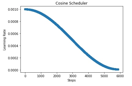
In our case, we have created a cosine scheduler with an initial learning rate of 0.001, the final learning rate of 1e-5, and the number of steps set to total batches of the training process. After completion of training, we have evaluated accuracy and classification report on test predictions as usual.
In the cell after accuracy calculation, we have plotted how the learning rate changes during training if we use a cosine scheduler.
from mxnet import gluon
from mxnet.gluon import loss
from mxnet import autograd
from mxnet import optimizer
from mxnet import lr_scheduler

batch_size=256
epochs=25
learning_rate = 0.001

model = CNN()
model.initialize()
loss_func = loss.SoftmaxCrossEntropyLoss()

steps = (X_train.shape[0]//batch_size)*epochs + epochs
scheduler = lr_scheduler.CosineScheduler(max_update=steps, base_lr=learning_rate, final_lr=1e-5)
grad_descent = optimizer.SGD(lr_scheduler=scheduler)

trainer = gluon.Trainer(model.collect_params(), grad_descent)

TrainModelInBatches(trainer, X_train, Y_train, X_test, Y_test, epochs, batch_size=batch_size)
from sklearn.metrics import accuracy_score, confusion_matrix, classification_report

Y_test_preds = model(X_test)
Y_test_preds = Y_test_preds.argmax(axis=-1)

print("Test Accuracy : {}".format(accuracy_score(Y_test_preds.asnumpy(), Y_test.asnumpy())))
print("Classification Report : ")
print(classification_report(Y_test_preds.asnumpy(), Y_test.asnumpy(), target_names=class_labels))
import matplotlib.pyplot as plt

scheduler = lr_scheduler.CosineScheduler(max_update=steps, base_lr=learning_rate, final_lr=1e-5)

lrs = [scheduler(i) for i in range(steps)]
plt.scatter(range(steps), lrs)
plt.title('Cosine Scheduler')
plt.xlabel("Steps")
plt.ylabel("Learning Rate");
6. Custom Scheduler (Combining Multiple Schedulers) 
In this section, we have explained how we can create a custom scheduler. We can create a custom scheduler as a class that has two methods implemented.
__init__()- This method has total logic to initialize scheduler.__call__()- This method takes iteration/step number as input and returns learning rate for that iteration/step.
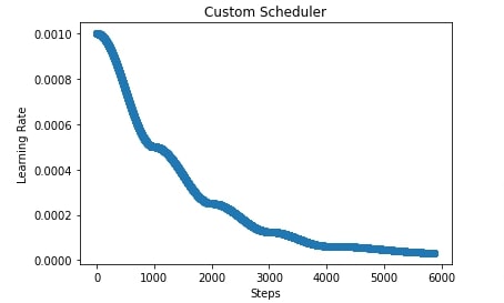
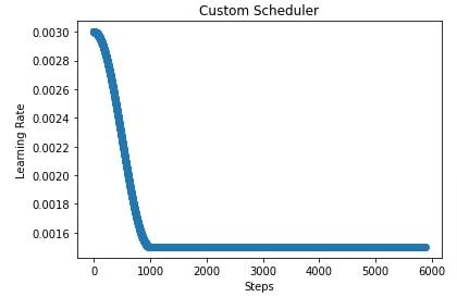
In our case below, we have created a scheduler that takes two parameters as input. The initial learning rate and boundaries parameter. The boundaries parameter accept a list of integer specifying boundaries of changing learning rate. The scheduler then creates cosine schedulers based on the length of boundaries parameters. If boundaries have 3 integers then it creates 4 cosine schedulers, if it has 4 integers then it creates 5 cosine schedulers. The first cosine scheduler has a base learning rate set to the initial learning rate and a final learning rate set to half of the initial learning rate. The second cosine scheduler has a base learning rate to the final learning rate of the previous cosine scheduler and the final learning rate is set to half of the final learning rate of the previous scheduler. The same process goes for all upcoming schedulers where we keep on halving the learning rate.
This example can also be considered as an example of how we can combine multiple schedulers in mxnet.
In the next two cells, we have explained for example how the learning rate will change if we use our custom scheduler.
class CustomScheduler:
    def __init__(self, base_lr=0.001, boundaries=None):
        self.base_lr = base_lr
        self.boundaries = boundaries
        if boundaries:
            self.schedulers = [lr_scheduler.CosineScheduler(max_update=self.boundaries[0], base_lr=self.base_lr, final_lr=self.base_lr/2)]
            self.base_lr = self.base_lr / 2
            for i in range(1, len(self.boundaries)):
                k = self.boundaries[i]-self.boundaries[i-1]
                scheduler = lr_scheduler.CosineScheduler(max_update=k, base_lr=self.base_lr, final_lr=self.base_lr/2)
                self.schedulers.append(scheduler)
                self.base_lr = self.base_lr/2
            scheduler = lr_scheduler.CosineScheduler(max_update=2000, base_lr=self.base_lr, final_lr=self.base_lr/2)
            self.schedulers.append(scheduler)
        else:
            self.schedulers = [lr_scheduler.CosineScheduler(max_update=1000, base_lr=self.base_lr, final_lr=self.base_lr/2)]

    def __call__(self, iteration):
        if self.boundaries:
            if iteration <= self.boundaries[0]:
                return self.schedulers[0](iteration)
            elif iteration > self.boundaries[-1]:
                return self.schedulers[-1](iteration-self.boundaries[-1])
            else:
                for i in range(1, len(self.boundaries)):
                    if iteration > self.boundaries[i-1] and iteration <= self.boundaries[i]:
                        return self.schedulers[i](iteration-self.boundaries[i-1])
        else:
            return self.schedulers[-1](iteration)
scheduler = CustomScheduler(base_lr=0.001, boundaries=[1000,2000,3000,4000])

scheduler.schedulers
for s in scheduler.schedulers:
    print(s.base_lr, s.final_lr)
In the below cell, we have initialized our custom scheduler with an initial learning rate of 0.001 and boundaries set to [1000,2000,3000,4000]. This will create 5 cosine schedulers that will anneal learning rate as per boundaries parameter.
In the cell after the below cell, we have plotted a chart showing how the learning rate will change during training if we use our custom scheduler.
from mxnet import gluon
from mxnet.gluon import loss
from mxnet import autograd
from mxnet import optimizer
from mxnet import lr_scheduler

batch_size=256
epochs=25
learning_rate = 0.001

model = CNN()
model.initialize()
loss_func = loss.SoftmaxCrossEntropyLoss()

steps = (X_train.shape[0]//batch_size)*epochs + epochs
scheduler = CustomScheduler(base_lr=0.001, boundaries=[1000,2000,3000,4000])
grad_descent = optimizer.SGD(lr_scheduler=scheduler)

trainer = gluon.Trainer(model.collect_params(), grad_descent)

TrainModelInBatches(trainer, X_train, Y_train, X_test, Y_test, epochs, batch_size=batch_size)
from sklearn.metrics import accuracy_score, confusion_matrix, classification_report

Y_test_preds = model(X_test)
Y_test_preds = Y_test_preds.argmax(axis=-1)

print("Test Accuracy : {}".format(accuracy_score(Y_test_preds.asnumpy(), Y_test.asnumpy())))
print("Classification Report : ")
print(classification_report(Y_test_preds.asnumpy(), Y_test.asnumpy(), target_names=class_labels))
import matplotlib.pyplot as plt

scheduler = CustomScheduler(base_lr=0.001, boundaries=[1000,2000,3000,4000])

lrs = [scheduler(i) for i in range(steps)]
plt.scatter(range(steps), lrs)
plt.title('Custom Scheduler')
plt.xlabel("Steps")
plt.ylabel("Learning Rate");
import matplotlib.pyplot as plt

scheduler = CustomScheduler(base_lr=0.003)

lrs = [scheduler(i) for i in range(steps)]
plt.scatter(range(steps), lrs)
plt.title('Custom Scheduler')
plt.xlabel("Steps")
plt.ylabel("Learning Rate");
This ends our small tutorial explaining how we can use learning rate schedulers available from mxnet to anneal learning rate during training. Please feel free to let us know your views in the comments section.
References
 Sunny Solanki
Sunny Solanki
Intro: Software Developer | Youtuber | Bonsai Enthusiast
About: Sunny Solanki holds a bachelor's degree in Information Technology (2006-2010) from L.D. College of Engineering. Post completion of his graduation, he has 8.5+ years of experience (2011-2019) in the IT Industry (TCS). His IT experience involves working on Python & Java Projects with US/Canada banking clients. Since 2020, he’s primarily concentrating on growing CoderzColumn.
His main areas of interest are AI, Machine Learning, Data Visualization, and Concurrent Programming. He has good hands-on with Python and its ecosystem libraries.
Apart from his tech life, he prefers reading biographies and autobiographies. And yes, he spends his leisure time taking care of his plants and a few pre-Bonsai trees.
Contact: sunny.2309@yahoo.in


![YouTube Subscribe]() Comfortable Learning through Video Tutorials?
Comfortable Learning through Video Tutorials?
If you are more comfortable learning through video tutorials then we would recommend that you subscribe to our YouTube channel.
![Need Help]() Stuck Somewhere? Need Help with Coding? Have Doubts About the Topic/Code?
Stuck Somewhere? Need Help with Coding? Have Doubts About the Topic/Code?
 Stuck Somewhere? Need Help with Coding? Have Doubts About the Topic/Code?
When going through coding examples, it's quite common to have doubts and errors.
If you have doubts about some code examples or are stuck somewhere when trying our code, send us an email at coderzcolumn07@gmail.com. We'll help you or point you in the direction where you can find a solution to your problem.
You can even send us a mail if you are trying something new and need guidance regarding coding. We'll try to respond as soon as possible.
![Share Views]() Want to Share Your Views? Have Any Suggestions?
Want to Share Your Views? Have Any Suggestions?
 Want to Share Your Views? Have Any Suggestions?
If you want to
- provide some suggestions on topic
- share your views
- include some details in tutorial
- suggest some new topics on which we should create tutorials/blogs
 mxnet, learning-rate-schedulers