PyTorch: Grad-CAM
Nowadays, getting good accuracy on computer vision tasks has become quite common due to convolutional neural networks. The models are easily generating more than 90% accuracy on tasks like image classification which was once quite hard to achieve. Though, many times, a high accuracy model does not necessarily mean that model has generalized well and uses patterns correct patterns from data to make predictions. Such models that have not generalized well fail miserably in production. Hence, to avoid a situation like that, we need a way to understand that our model is actually using parts of the sample that it should use for making predictions. To give an example, let's say that we have an image classification task of classifying cat vs dog, then our model should be activating on parts of the image where there is a cat or dog and not on some background. If we can get information about which parts our model is activating then we can be more confident about the performance of our network that it is using the right patterns to make predictions.
To our surprise, an algorithm named Grad-CAM (Gradient-weighted Class Activation Mapping) is developed that let us look at parts of the image that contributed to the prediction. The grad-CAM algorithm uses the gradients of any target (say 'cat' in a classification network) flowing into the final convolution layer to produce a coarse localization map highlighting the important regions in the image for predicting the concept. Basically, it highlights activations that contributed most to predicting the particular category using gradients of the last convolution layer with respect to predicted output. The output of the grad-CAM algorithm is a heatmap with the same shape as that of an image which we can overlay over the image to see which parts of the image contributed to the prediction. Below, we have highlighted the steps of the grad-CAM algorithm.
Steps of Grad-CAM
- Capture the output of the last convolution layer of the network.
- Take gradient of last convolution layer with respect to prediction probability. (We can take predictions with respect to any class we want. In our case, we'll take prediction with the highest probability. We can look at other probabilities as well)
- Average gradients calculated in the previous step at axis which has the same dimension as output channels of last convolution layer. The output of this step will be 1D array that has the same numbers as that of output channels of the last convolution layer.
- Multiply convolution layer output with averaged gradients from the previous step at output channel level, i.e. first channel output should be multiplied with first averaged value, second should be multiplied with the second value, and so on.
- Average output from the previous step at channel level to create 2D heatmap that has the same dimension as that of image.
- Normalize heatmap (Optional step but recommended as it helps improve results).
The steps will become more clear when we explain with an example below.
As a part of our tutorial, we have used the Fashion MNIST dataset and trained a simple convolutional neural network of 3 convolution layers on it. The network is designed using PyTorch. We have tried to keep things simple for the reader to understand how the algorithm works and how individuals can code it for their task. After getting good accuracy using our model, we have explained the prediction using the Grad-CAM algorithm by showing step by step process.
Below are important sections of tutorial to give an overview of the material covered.
- Load Dataset
- Define CNN
- Train Network
- Grad-CAM
- Explain Correct Predictions Using Last Convolution Layer (Step By Step Algorithm)
- Explain Correct Prediction Using Second Last Convolution Layer
- Explain Correct Prediction Using Third Last Convolution Layer
Below, we have imported PyTorch and printed the version of it that we have used in our tutorial.
import torch

print("PyTorch Version : {}".format(torch.__version__))
Load Dataset 
In this section, we have loaded the Fashion MNIST dataset available from keras. The dataset has grayscale images of shape (28,28) pixels for 10 different fashion items. The dataset is already divided into a train (60k images) and test (10k images) sets. After loading datasets, we have converted them to PyTorch tensors. Then, we have created tensor datasets and data loaders for looping through data easily in bathes during training. We'll be using these data loaders during training. Below, we have included mapping from the target class index to the target class name.
| Label | Description |
|---|---|
| 0 | T-shirt/top |
| 1 | Trouser |
| 2 | Pullover |
| 3 | Dress |
| 4 | Coat |
| 5 | Sandal |
| 6 | Shirt |
| 7 | Sneaker |
| 8 | Bag |
| 9 | Ankle boot |
from tensorflow import keras
from sklearn.model_selection import train_test_split

(X_train, Y_train), (X_test, Y_test) = keras.datasets.fashion_mnist.load_data()

X_train, X_test, Y_train, Y_test = torch.tensor(X_train, dtype=torch.float32),\
                                   torch.tensor(X_test, dtype=torch.float32),\
                                   torch.tensor(Y_train, dtype=torch.long),\
                                   torch.tensor(Y_test, dtype=torch.long)

X_train, X_test = X_train.reshape(-1,1,28,28), X_test.reshape(-1,1,28,28)

X_train, X_test = X_train/255.0, X_test/255.0

classes =  Y_train.unique()
class_labels = ["T-shirt/top","Trouser","Pullover","Dress","Coat","Sandal","Shirt","Sneaker","Bag","Ankle boot"]
mapping = dict(zip(classes.numpy(), class_labels))

X_train.shape, X_test.shape, Y_train.shape, Y_test.shape
mapping
from torch.utils.data import TensorDataset, DataLoader

train_dataset = TensorDataset(X_train, Y_train)
test_dataset  = TensorDataset(X_test , Y_test)

train_loader = DataLoader(train_dataset, batch_size=128, shuffle=True)
test_loader = DataLoader(test_dataset, batch_size=128, shuffle=True)
Define CNN 
Here, we have defined the network that we'll use to classify images. We have designed a simple convolutional neural network using PyTorch. The network has 3 convolution layers and one linear layer. The convolution layers have 48, 32, and 16 output channels respectively. All of them have relu activation function. The last linear layer has 10 output units which are the same as the number of target classes.
Please make a NOTE that we have not covered how to design a network using PyTorch in detail. Please feel free to check the below links if you want a background with it.
from torch import nn
import torch.nn.functional as F

class ConvNet(nn.Module):
    def __init__(self):
        super(ConvNet, self).__init__()
        self.seq = nn.Sequential(
            nn.Conv2d(in_channels=1, out_channels=48, kernel_size=(3,3), padding="same"),
            nn.ReLU(),

            nn.Conv2d(in_channels=48, out_channels=32, kernel_size=(3,3), padding="same"),
            nn.ReLU(),

            nn.Conv2d(in_channels=32, out_channels=16, kernel_size=(3,3), padding="same"),
            nn.ReLU(),

            nn.Flatten(),
            nn.Linear(16*28*28, len(classes)),
            #nn.Softmax(dim=1)
        )

    def forward(self, x_batch):
        preds = self.seq(x_batch)
        return preds

conv_net = ConvNet()

conv_net
Train Network 
In this section, we have trained our network on data. We have created a simple training function. The function takes model, loss function, optimizer, train loader, validation loaded, and epochs as input. It then executes the training loop number of epoch times. Each time, it loops through whole training data in batches using train data loader. During each batch, it performs a forward pass to make predictions, calculates loss using predictions & actual targets, calculate gradients, and update network parameters using gradients. It keeps track of loss during each batch and prints average loss after completion of an epoch. It also calculates validation loss and validation accuracy after each epoch and prints it. We have created helper functions to make predictions and calculate the loss for validation data.
from sklearn.metrics import accuracy_score
from tqdm import tqdm
import gc

def CalcValLoss(model, loss_func, val_loader):
    with torch.no_grad(): ## Prevents calculation of gradients
        val_losses = []
        for X_batch, Y_batch in val_loader:
            preds = model(X_batch)
            loss = loss_func(preds, Y_batch)
            val_losses.append(loss)
        print("Valid CategoricalCrossEntropy : {:.3f}".format(torch.tensor(val_losses).mean()))

def MakePredictions(model, loader):
    preds, Y_shuffled = [], []
    for X_batch, Y_batch in loader:
        preds.append(model(X_batch))
        Y_shuffled.append(Y_batch)

    preds = torch.cat(preds).argmax(axis=-1)
    Y_shuffled = torch.cat(Y_shuffled)
    return Y_shuffled, preds

def TrainModelInBatchesV1(model, loss_func, optimizer, train_loader, val_loader, epochs=5):
    for i in range(epochs):
        losses = [] ## Record loss of each batch
        for X_batch, Y_batch in tqdm(train_loader):
            preds = model(X_batch) ## Make Predictions by forward pass through network

            loss = loss_func(preds, Y_batch) ## Calculate Loss
            losses.append(loss) ## Record Loss

            optimizer.zero_grad() ## Zero weights before calculating gradients
            loss.backward() ## Calculate Gradients
            optimizer.step() ## Update Weights

        print("Train CategoricalCrossEntropy : {:.3f}".format(torch.tensor(losses).mean()))
        CalcValLoss(model, loss_func, val_loader)

        Y_test_shuffled, test_preds = MakePredictions(model, val_loader)
        val_acc = accuracy_score(Y_test_shuffled, test_preds)
        print("Val  Accuracy : {:.3f}".format(val_acc))
        gc.collect()
Below, we have actually trained our network using the training function defined in the previous cell. We have initialized a number of epochs to 5 and the learning rate to 0.001. Then, we have initialized the network, initialized cross entropy loss, and Adam optimizer. At last, we have called our training routine to perform training. We can notice from the loss and accuracy getting printed after each epoch that our model is doing a good job at the image classification task. Now, in the next section, we can actually verify which parts of images are contributing to prediction using Grad-CAM algorithm.
from torch.optim import SGD, RMSprop, Adam

#torch.manual_seed(42) ##For reproducibility.This will make sure that same random weights are initialized each time.
epochs = 5
learning_rate = torch.tensor(1e-3) # 0.001

conv_net = ConvNet()
cross_entropy_loss = nn.CrossEntropyLoss()
optimizer = Adam(params=conv_net.parameters(), lr=learning_rate)

TrainModelInBatchesV1(conv_net, cross_entropy_loss, optimizer, train_loader, test_loader,epochs)
Grad-CAM 
In this section, we'll try to explain the prediction made by our model using Grad-CAM algorithm. We have first explained the whole process step by step by executing each step individually and then we have created a simple function to execute them all together.
Explain Correct Predictions Using Last Convolution Layer (Step By Step Algorithm)
In this section, we have explained how we can use Grad-CAM for the last convolution layer. The reason behind this is that the last convolution layer generally combines the patterns of previous convolution layers to create a final pattern that will contribute to the prediction. We'll later perform Grad-CAM with respect to other convolution layers as well to understand their contributions.
1. Capture Output Of Last Convolution Layer
As a part of our first step, we have captured the output of the last convolution layer. In order to do that we have designed a second convolution network using layers of our original CNN. We can retrieve the layers of our original network by calling children() function on the network. Then, we have created another network that performs the same forward pass as our original network using layers of our original network. But it captures the output of the last convolution layer which we need for our purpose. It keeps the output as one of its local members.
After creating a new network to capture the last Conv layer output, we have randomly selected one sample from test data and performed a forward pass through the network using this sample. The output of this network is the same as our original network which is 10 probabilities per sample. We can notice that the output of the last Conv layer is of shape (1,16,28,28) where 16 is the output channels of the conv layer and batch size is 1 because we have taken a single sample into consideration.
We have also printed the actual and predicted labels of the selected sample.
list(conv_net.children())[0]
class LastConvLayerModel(nn.Module):
    def __init__(self):
        super(LastConvLayerModel, self).__init__()
        self.layers = list(list(conv_net.children())[0].children())

    def forward(self, X_batch):
        x = self.layers[0](X_batch)
        conv_layer_output = None
        for i, layer in enumerate(self.layers[1:]):
            x = layer(x)
            if i == 3: ## Output after 3rd Convolution layer
                self.conv_layer_output = x
        return x
import numpy as np

conv_model = LastConvLayerModel()
idx = np.random.choice(range(10000))
pred = conv_model(X_test[idx:idx+1])

F.softmax(pred, dim=-1).argmax(), F.softmax(pred, dim=-1).max()
conv_model.conv_layer_output.shape
print("Actual    Target : {}".format(mapping[Y_test[idx].item()]))
print("Predicted Target : {}".format(mapping[pred.argmax(dim=-1).item()]))
2. Take Gradients Of Last Conv Layer Output With Respect to Prediction
In this section, we have calculated the gradient of the last convolution layer output with respect to the predicted item. We have used grad() function from autograd sub-module of PyTorch for our purpose. The first value to the function is predicted probability and the second value is an output of the last convolution layer. The function then calculates gradients and returns them. We can notice that the output shape of the gradient is (1,16,28,28) same as the last convolution layer output shape.
Please make a NOTE below that we are taking gradients with respect to the maximum predicted probability below. We can take gradients with respect to any probability out of 10 probability if we want to check activations for other target classes.
from torch import autograd

grads = autograd.grad(pred[:, pred.argmax().item()], conv_model.conv_layer_output)

grads[0].shape
3. Average Gradients
In this section, we have averaged gradients at the output channel level to get average gradients per channel. We have taken gradients at axis (0,2,3) which will return gradients array of shape 16 which is the same as the output channels of the last convolution layer.
pooled_grads = grads[0].mean((0,2,3))

pooled_grads
4. Multiply Convolution Layer Output with Averaged Gradients
In this section, we have multiplied the output of the last convolution layer with averaged gradients from the previous section. We have looped through each channel of the last Conv layer output and multiplied them with the averaged gradient at that channel. This will generate an output of shape (16,28,28).
conv_output = conv_model.conv_layer_output.squeeze()

conv_output = F.relu(conv_output)

conv_output.shape
for i in range(len(pooled_grads)):
    conv_output[i,:,:] *= pooled_grads[i]

conv_output.shape
5. Average Output At Channel Axis To Create Heatmap
This is our last step where we have taken the average at the channel level (16 channels) on the output of the previous step. This will generate a heatmap of shape (28,28) which will have activations that contribute to the predictions. We generally normalize the outputs of the heatmap for better results.
heatmap = conv_output.mean(dim=0).squeeze()

## Normalize heatmap
#heatmap = F.relu(heatmap) / torch.max(heatmap)
heatmap = heatmap / torch.max(heatmap)

heatmap.shape
6. Visualize Original Image And Heatmap
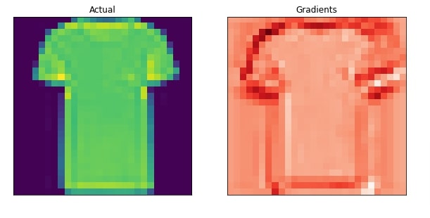
In this section, we have visualized our original image and heatmap next to each other to understand the performance of Grad-CAM algorithm. We can notice from the results that the heatmap highlights activations that contributed to the prediction.
import matplotlib
import matplotlib.pyplot as plt

def plot_actual_and_heatmap(idx, heatmap):
    cmap = matplotlib.cm.get_cmap("Reds")

    fig = plt.figure(figsize=(10,10))
    ax1 = fig.add_subplot(121)
    ax1.imshow(X_test[idx].numpy().squeeze());
    ax1.set_title("Actual");
    ax1.set_xticks([],[]);ax1.set_yticks([],[]);

    ax2 = fig.add_subplot(122)
    ax2.imshow(heatmap, cmap="Reds");
    ax2.set_title("Gradients");
    ax2.set_xticks([],[]);ax2.set_yticks([],[]);

plot_actual_and_heatmap(idx, heatmap.detach())

Explain Correct Prediction Using Second Last Convolution Layer
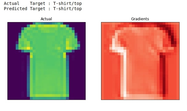
In this section, we have tried to explain the predictions using the output of the second last convolution layer with our Grad-CAM algorithm. As usual, we have created a network that captures the output of the second-last convolution layer. Then, we have created a method that executes steps of Grad-CAM algorithm that we had explained separately earlier.
At last, we have called our method to generate a heatmap for the input sample and visualized it along with an actual image.
class ConvLayerModel(nn.Module):
    def __init__(self):
        super(ConvLayerModel, self).__init__()
        self.layers = list(list(conv_net.children())[0].children())

    def forward(self, X_batch):
        x = self.layers[0](X_batch)
        for i, layer in enumerate(self.layers[1:]):
            x = layer(x)
            if i == 1: ## Output after 2nd Convolution layer
                self.conv_layer_output = x
        return x
def calculate_gradcam_heatmap(idx):
    conv_model = ConvLayerModel()
    pred = conv_model(X_test[idx:idx+1]) ## Make Prediction using Model

    print("Actual    Target : {}".format(mapping[Y_test[idx].item()]))
    print("Predicted Target : {}".format(mapping[pred.argmax(dim=-1).item()]))

    grads = autograd.grad(pred[:, pred.argmax().item()], conv_model.conv_layer_output) ## Calculate Gradients with respect to predicted class

    pooled_grads = grads[0].mean((0,2,3)) ## Average Gradients

    conv_output = conv_model.conv_layer_output.squeeze().detach()  ## Remove Extra Dimension From begining
    conv_output = F.relu(conv_output) ## Apply Relu
    for i in range(len(pooled_grads)):
        conv_output[i,:,:] *= pooled_grads[i] ## Multiply channel-wise convolution layer output with average gradients.

    heatmap = conv_output.mean(dim=0).squeeze() ## Average Gradients across all channels and remove extra dimension.

    #heatmap = (heatmap - heatmap.min()) / (heatmap.max() - heatmap.min())
    #heatmap = F.relu(heatmap) / torch.max(heatmap)  ## Normalize heatmap
    heatmap = heatmap / torch.max(heatmap)  ## Normalize heatmap

    return heatmap.detach()
heatmap = calculate_gradcam_heatmap(idx)
plot_actual_and_heatmap(idx, heatmap)

Explain Correct Prediction Using Third Last Convolution Layer
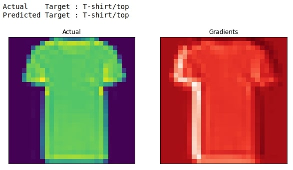
In this section, we have calculated Grad-CAM heatmap using our third last convolution layer which actually the first convolution layer in our network. This will help us see what patterns are contributing from the first convolution layer for prediction.
We have designed a network that captures the output of the first convolution layer. Then, we have called our method to perform steps of the Grad-CAM algorithm to generate a heatmap for our sample. At last, we have plotted the actual image and heatmap next to each other for comparison.
class ConvLayerModel(nn.Module):
    def __init__(self):
        super(ConvLayerModel, self).__init__()
        self.layers = list(list(conv_net.children())[0].children())

    def forward(self, X_batch):
        x = self.layers[0](X_batch)
        self.conv_layer_output = x
        for i, layer in enumerate(self.layers[1:]):
            x = layer(x)
        return x
heatmap = calculate_gradcam_heatmap(idx)
plot_actual_and_heatmap(idx, heatmap)

gc.collect()
This ends our small tutorial explaining how we can design our Grad-CAM algorithm with PyTorch network. Please feel free to let us know your views in the comments section.
References
 Sunny Solanki
![YouTube Subscribe]() Comfortable Learning through Video Tutorials?
Comfortable Learning through Video Tutorials?
If you are more comfortable learning through video tutorials then we would recommend that you subscribe to our YouTube channel.
![Need Help]() Stuck Somewhere? Need Help with Coding? Have Doubts About the Topic/Code?
Stuck Somewhere? Need Help with Coding? Have Doubts About the Topic/Code?
When going through coding examples, it's quite common to have doubts and errors.
If you have doubts about some code examples or are stuck somewhere when trying our code, send us an email at coderzcolumn07@gmail.com. We'll help you or point you in the direction where you can find a solution to your problem.
You can even send us a mail if you are trying something new and need guidance regarding coding. We'll try to respond as soon as possible.
![Share Views]() Want to Share Your Views? Have Any Suggestions?
Want to Share Your Views? Have Any Suggestions?
If you want to
- provide some suggestions on topic
- share your views
- include some details in tutorial
- suggest some new topics on which we should create tutorials/blogs


 Comfortable Learning through Video Tutorials?
 Stuck Somewhere? Need Help with Coding? Have Doubts About the Topic/Code?
 Want to Share Your Views? Have Any Suggestions?
 pytorch, grad-CAM, image-classification