SHAP Values for Image Classification Tasks (Keras)
Deep learning models like convolutional neural networks are giving quite good results at many computer vision tasks. We need to understand that the models that are giving such high accuracy are predicting results based on data parts that they should use for prediction. Let's say for example that we have an image classification task of predicting cat vs dog then the model should look at pixels of face and body of cat/dog to predict class, not the background pixels of images should be used to make a decision. If that is the case then we can be sure that our model has generalized better and actually learning features of cats and dogs. There are many prediction interpretation libraries but as a part of this tutorial, we'll be using SHAP. SHAP is a python library that generates shap values for predictions using a game-theoretic approach. We can then visualize these shap values using various visualizations to understand which features contributed to prediction. We have a starter tutorial on SHAP where we discuss how to use it for tabular (structured) datasets. Please check the below link if you want to refer to it.
As a part of this tutorial, we have designed a simple CNN using keras and trained it with the Fashion MNIST dataset. Then, we have explained correct and incorrect predictions using SHAP python library.
Below, we have listed important sections of tutorial to give an overview of the material covered.
Important Sections Of Tutorial
- Load Data
- Define CNN
- Compile And Train Model
- Evaluate Model Performance
- Explain Predictions Using SHAP Partition Explainer
- Visualize SHAP Values For Correct Predictions
- Image Plots
- Visualize SHAP Values For Incorrect Predictions
- Visualize SHAP Values For Correct Predictions
- Explain Predictions Using SHAP Permutation Explainer
- Visualize SHAP Values For Correct Predictions
- Visualize SHAP Values For Incorrect Predictions
Below, we have imported the necessary libraries and printed the versions that we have used in our tutorial.
import tensorflow
from tensorflow import keras

print("Keras Version : {}".format(keras.__version__))
import shap

print("SHAP Version : {}".format(shap.__version__))
1. Load Data 
In this section, we have loaded the Fashion MNIST dataset available from keras. The dataset has grayscale images of shape (28,28) pixels for 10 different fashion items. The dataset is already divided into the train (60k images) and test (10k images) sets. Below we have included mapping from index to fashion item names.
| Label | Description |
|---|---|
| 0 | T-shirt/top |
| 1 | Trouser |
| 2 | Pullover |
| 3 | Dress |
| 4 | Coat |
| 5 | Sandal |
| 6 | Shirt |
| 7 | Sneaker |
| 8 | Bag |
| 9 | Ankle boot |
from tensorflow import keras
from sklearn.model_selection import train_test_split
from jax import numpy as jnp
import numpy as np

(X_train, Y_train), (X_test, Y_test) = keras.datasets.fashion_mnist.load_data()

X_train, X_test = X_train.reshape(-1,28,28,1), X_test.reshape(-1,28,28,1)

X_train, X_test = X_train/255.0, X_test/255.0

classes =  np.unique(Y_train)
class_labels = ["T-shirt/top","Trouser","Pullover","Dress","Coat","Sandal","Shirt","Sneaker","Bag","Ankle boot"]
mapping = dict(zip(classes, class_labels))

X_train.shape, X_test.shape, Y_train.shape, Y_test.shape
2. Define CNN 
In this section, we have defined a convolutional neural network that we'll use to classify images of the Fashion MNIST dataset loaded earlier. The network is simple with 2 convolution layers and one dense layer. The two convolution layers have filters 32 and 16 respectively and both are using kernel size of (3,3). We have applied relu (rectified linear unit) activation after both convolution layers. The output of the second convolution layer is flattened and then given to the dense layer. The dense layer has 10 output units, the same as the number of target classes.
from tensorflow.keras.models import Sequential
from tensorflow.keras import layers

model = Sequential([
    layers.Input(shape=X_train.shape[1:]),
    layers.Conv2D(filters=32, kernel_size=(3,3), padding="same", activation="relu"),
    layers.Conv2D(filters=16, kernel_size=(3,3), padding="same", activation="relu"),

    layers.Flatten(),
    layers.Dense(len(classes), activation="softmax")
])

model.summary()
3. Compile And Train Model 
In this section, we have first compiled our model to use Adam optimizer, cross entropy loss, and accuracy metric. Then, we have trained the model for 10 epochs using train and validation data. We can notice from the results getting printed after each epoch that the model has achieved near 91% accuracy on validation data and 93% accuracy on train data. It seems to be good accuracy and we can now evaluate the predictions made by our model.
model.compile("adam", "sparse_categorical_crossentropy", ["accuracy"])
model.fit(X_train, Y_train, batch_size=256, epochs=10, validation_data=(X_test, Y_test))
4. Evaluate Model Performance 
In this section, we have evaluated the performance of our network by calculating accuracy, confusion matrix, and classification report (precision, recall, and f1-score per class) metrics. We can notice from the results that our model is doing good for categories except 'shirt', 'coat', 'pullover' and 'top' which are almost the same hence can be confusing for the model to differentiate between them in grayscale images. Many 'shirt' category images are confused with 't-shirt/top' category as there is quite less difference between them.
We have used the function available from scikit-learn to calculate various metrics. If you want to learn about various ML metrics available from sklearn then please feel free to check the below link which covers the majority of them.
from sklearn.metrics import accuracy_score, confusion_matrix, classification_report

Y_test_preds = model.predict(X_test)
Y_test_preds = np.argmax(Y_test_preds, axis=1)

print("Test Accuracy : {}".format(accuracy_score(Y_test, Y_test_preds)))
print("\nConfusion Matrix : ")
print(confusion_matrix(Y_test, Y_test_preds))
print("\nClassification Report :")
print(classification_report(Y_test, Y_test_preds, target_names=class_labels))
5. SHAP Partition Explainer 
In this section, we have used SHAP partition explainer to explain the predictions made by our network. We have tried to explain both correct and wrong predictions of our model to see which parts of an image are contributing to predictions.
In order to use SHAP, we first need to initialize it by calling initjs() function.
Then, we have created an instance of Partition explainer by using Explainer() constructor. We have given three values to the constructor.
- Our trained model
- Masker to mask parts of an image using blurring or inpainting.
- List of Target Class labels
The Explainer() constructor by default creates an instance of Partition explainer. We can generate shap values for images using this explainer object.
shap.initjs()

masker = shap.maskers.Image("inpaint_telea", X_train[0].shape)

explainer = shap.Explainer(model, masker, output_names=class_labels)

explainer
Visualize SHAP Values For Correct Predictions
In this section, we have explained the correct predictions made by our model. We have first taken 4 sample images from our test dataset and generated shap values for them using the partition explainer object we created earlier. Then, we have printed the actual labels, predicted labels, and the model's predicted probabilities.
shap_values = explainer(X_test[:4], outputs=shap.Explanation.argsort.flip[:5])

shap_values.shape
print("Actual Labels    : {}".format([mapping[i] for i in Y_test[:4]]))
probs = model.predict(X_test[:4])
print("Predicted Labels : {}".format([mapping[i] for i in np.argmax(probs, axis=1)]))
print("Probabilities : {}".format(np.max(probs, axis=1)))
Image Plot
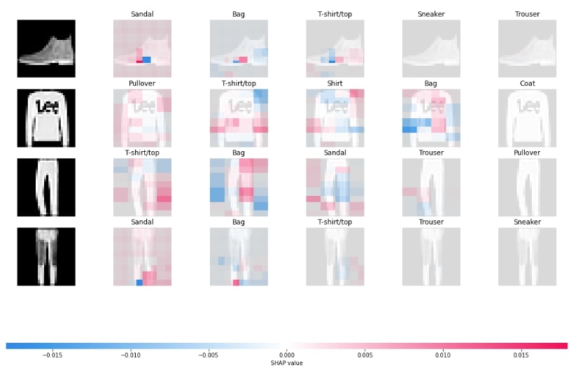
In this section, we have generated image plots that visualizes shap values generated by the explainer object.
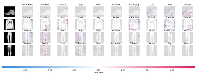
Below, we have generated the first image plot using shap values generated in previous cells. The chart shows the actual image and parts of it highlighted in shades of red and blue colors. The shades of red color show parts that contributed positively and shades of blue color show parts that contributed negatively to the prediction of that category. It also shows the first five categories that the model thinks the image belongs to.
shap.image_plot(shap_values)
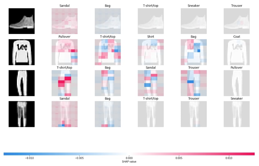
Below, we have generated another image plot using a different masker named inpaint_ns. We have created masker and explainer instances for this again.
masker = shap.maskers.Image("inpaint_ns", X_train[0].shape)

explainer = shap.Explainer(model, masker, output_names=class_labels)

shap_values = explainer(X_test[:4], outputs=shap.Explanation.argsort.flip[:5])

shap.image_plot(shap_values)
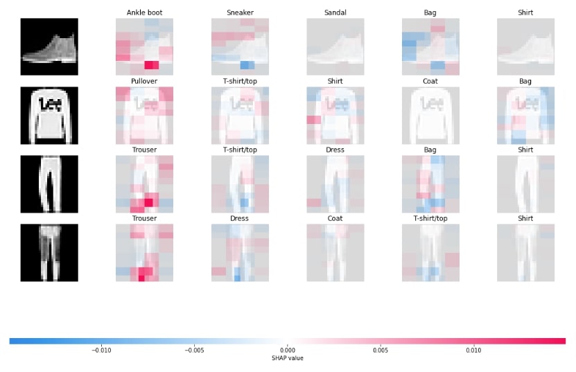
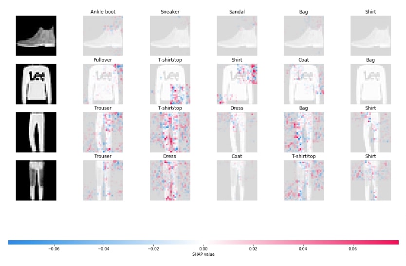
Below, we have generated another image plot using masker that uses blurring-based masker. We can notice that the blurring masker seems to be doing a good job compared to other maskers. The tuple of integer values that we provide in the string of masker is the size of the kernel used to blur.
masker = shap.maskers.Image("blur(28,28)", X_train[0].shape)

explainer = shap.Explainer(model, masker, output_names=class_labels)

shap_values = explainer(X_test[:4], outputs=shap.Explanation.argsort.flip[:5])

shap.image_plot(shap_values)
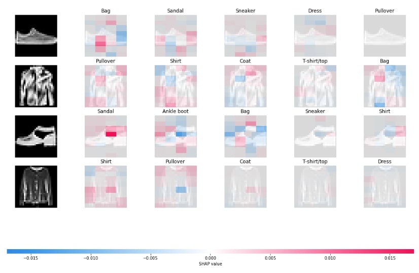
Visualize SHAP Values For Incorrect Predictions
In this section, we have explained wrong predictions using the explainer object. In order to explain wrong predictions, we have first retrieved indexes of all wrong predictions from the test set. Then, we have used indexes of wrong predictions to retrieve those samples and make predictions on them again to retrieve the probabilities of the model for those predictions.
wrong_preds_idx = np.argwhere(Y_test!=Y_test_preds)

X_batch = X_test[wrong_preds_idx.flatten()[:4]]
Y_batch = Y_test[wrong_preds_idx.flatten()[:4]]

print("Actual Labels    : {}".format([mapping[i] for i in Y_batch]))
probs = model.predict(X_batch)
print("Predicted Labels : {}".format([mapping[i] for i in np.argmax(probs, axis=1)]))
print("Probabilities : {}".format(np.max(probs, axis=1)))
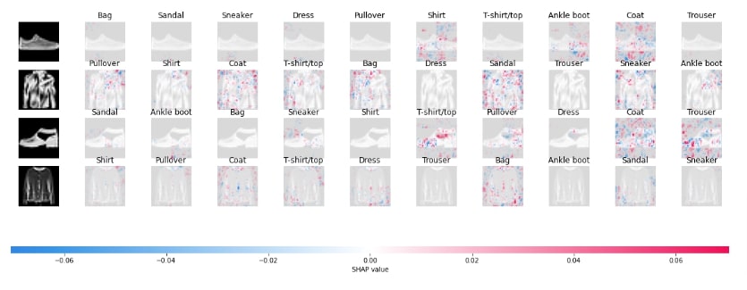
Below, we have generated an image plot using by generating shap values for wrong predictions. In the next cell, we have explained that we can generate visualization using image() function of plots sub-module of shap library.
masker = shap.maskers.Image("blur(28,28)", X_train[0].shape)

explainer = shap.Explainer(model, masker, output_names=class_labels)

shap_values = explainer(X_batch, outputs=shap.Explanation.argsort.flip[:5])

shap.image_plot(shap_values)
shap.plots.image(shap_values)
6. SHAP Permutation Explainer 
In this section, we are trying another explainer available from a shap named permutation explainer. The permutation explainer can be created using PermutationExplainer() constructor and accepts the same parameters as the permutation explainer. The permutation explainer tries different combinations of features to generate shap values.
Below, we have first created a permutation explainer using model and masker objects.
masker = shap.maskers.Image("blur(28,28)", X_train[0].shape)

explainer = shap.PermutationExplainer(model, masker, output_names=class_labels)

explainer
Visualize SHAP Values For Correct Predictions
In this section, we have generated shap values for 4 test images using the permutation explainer object. In the next cell, we have also printed actual labels, predicted labels, and probabilities of those 4 sample images. We have also calculated labels according to the 10 probabilities generated by our model.
shap_values = explainer(X_test[:4], max_evals=1600, outputs=shap.Explanation.argsort.flip[:5])

shap_values.shape
print("Actual Labels    : {}".format([mapping[i] for i in Y_test[:4]]))
probs = model.predict(X_test[:4])
print("Predicted Labels : {}".format([mapping[i] for i in np.argmax(probs, axis=1)]))
print("Probabilities : {}".format(np.max(probs, axis=1)))
Y_preds = model.predict(X_test[:4])

Y_preds = Y_preds.argsort()[:, ::-1]
Y_labels = [[class_labels[val] for val in row] for row in Y_preds]
Y_labels=np.array(Y_labels)

Y_labels
In this below cell, we have plotted an image plot showing shap values that contributed to predictions.
shap.image_plot(shap_values, labels=Y_labels)
shap.image_plot(shap_values[:,:,:,:,:5], labels=Y_labels[:,:5])
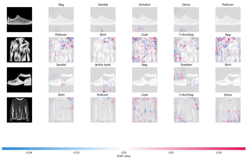
Visualize SHAP Values For Incorrect Predictions
In this section, we have generated shap values for wrong predictions. The majority of code in this section is a repeat of earlier sections hence we have not included repeated explanations for them.
wrong_preds_idx = np.argwhere(Y_test!=Y_test_preds)

X_batch = X_test[wrong_preds_idx.flatten()[:4]]
Y_batch = Y_test[wrong_preds_idx.flatten()[:4]]

print("Actual Labels    : {}".format([mapping[i] for i in Y_batch]))
probs = model.predict(X_batch)
print("Predicted Labels : {}".format([mapping[i] for i in np.argmax(probs, axis=1)]))
print("Probabilities : {}".format(np.max(probs, axis=1)))
masker = shap.maskers.Image("blur(28,28)", X_train[0].shape)

explainer = shap.PermutationExplainer(model, masker, output_names=class_labels)

shap_values = explainer(X_batch, max_evals=1600, outputs=shap.Explanation.argsort.flip[:5])

shap_values.shape
Y_preds = model.predict(X_batch)

Y_preds = Y_preds.argsort()[:, ::-1]
Y_labels = [[class_labels[val] for val in row] for row in Y_preds]
Y_labels=np.array(Y_labels)

Y_labels
shap.image_plot(shap_values, labels=Y_labels)
shap.image_plot(shap_values[:,:,:,:,:5], labels=Y_labels[:,:5])
This ends our small tutorial explaining how we can generate SHAP values for image classification networks created using keras to explain predictions made by the model. Please feel free to let us know your views in the comments section.
References
 Sunny Solanki
Sunny Solanki
Intro: Software Developer | Youtuber | Bonsai Enthusiast
About: Sunny Solanki holds a bachelor's degree in Information Technology (2006-2010) from L.D. College of Engineering. Post completion of his graduation, he has 8.5+ years of experience (2011-2019) in the IT Industry (TCS). His IT experience involves working on Python & Java Projects with US/Canada banking clients. Since 2020, he’s primarily concentrating on growing CoderzColumn.
His main areas of interest are AI, Machine Learning, Data Visualization, and Concurrent Programming. He has good hands-on with Python and its ecosystem libraries.
Apart from his tech life, he prefers reading biographies and autobiographies. And yes, he spends his leisure time taking care of his plants and a few pre-Bonsai trees.
Contact: sunny.2309@yahoo.in


![YouTube Subscribe]() Comfortable Learning through Video Tutorials?
Comfortable Learning through Video Tutorials?
If you are more comfortable learning through video tutorials then we would recommend that you subscribe to our YouTube channel.
![Need Help]() Stuck Somewhere? Need Help with Coding? Have Doubts About the Topic/Code?
Stuck Somewhere? Need Help with Coding? Have Doubts About the Topic/Code?
 Stuck Somewhere? Need Help with Coding? Have Doubts About the Topic/Code?
When going through coding examples, it's quite common to have doubts and errors.
If you have doubts about some code examples or are stuck somewhere when trying our code, send us an email at coderzcolumn07@gmail.com. We'll help you or point you in the direction where you can find a solution to your problem.
You can even send us a mail if you are trying something new and need guidance regarding coding. We'll try to respond as soon as possible.
![Share Views]() Want to Share Your Views? Have Any Suggestions?
Want to Share Your Views? Have Any Suggestions?
 Want to Share Your Views? Have Any Suggestions?
If you want to
- provide some suggestions on topic
- share your views
- include some details in tutorial
- suggest some new topics on which we should create tutorials/blogs
 shap-values, image-classification, keras