SHAP Values for Text Classification Tasks (Keras NLP)
SHAP (SHapley Additive exPlanations) is a Python library that uses a Game-theoretic approach to generate SHAP values which can be used to explain predictions made by our machine learning models. SHAP can be used to explain predictions for tasks related to fields like computer vision, natural language processing, structured data ML, etc. We have already covered a detailed tutorial about how it can be used for tabular datasets.
As a part of this tutorial, we'll be primarily concentrating on the text classification task of NLP. We'll be using 20 newsgroups text datasets available from scikit-learn. We have trained a simple neural network designed using Keras with a text dataset. Then, we have explained right and wrong predictions made by the model using SHAP values. We have created various visualizations explaining which words contributed to the predictions.
We have one more tutorial explaining how to use shap values to explain text classification models where we have used scikit-learn vectorizers to vectorize text data. Please feel free to check the below link if you want to have a look at that tutorial.
Below, we have listed important sections of tutorial to give an overview of the material covered.
Important Sections Of Tutorial
- Load Data
- Vectorize Text Data (Word Frequency)
- Create And Train Network
- Evaluate Model Performance
- Explain Model Predictions Using SHAP Partition Explainer
- Visualize SHAP Values For Correct Predictions
- Text Plots
- Bar Charts
- Waterfall Chart
- Force Plot
- Visualize SHAP Values For Incorrect Predictions
- Text Plots
- Bar Charts
- Force Plot
- Visualize SHAP Values For Correct Predictions
Below, we have imported important libraries of our tutorial and printed the version that we have used.
import tensorflow
from tensorflow import keras

print("Keras Version : {}".format(keras.__version__))
import shap

print("SHAP Version : {}".format(shap.__version__))
1. Load Data 
In this section, we have loaded 20 newsgroups dataset available from scikit-learn. The dataset has around 18k text documents for 20 different categories. We have limited our tutorial to using only 5 categories. This will make our problem a multi-class text classification problem. The dataset is loaded using fetch_20newsgroups() function available from datasets sub-module of scikit-learn. It let us load train and test sets separately.
import numpy as np
from sklearn import datasets

all_categories = ['alt.atheism','comp.graphics','comp.os.ms-windows.misc','comp.sys.ibm.pc.hardware',
                  'comp.sys.mac.hardware','comp.windows.x', 'misc.forsale','rec.autos','rec.motorcycles',
                  'rec.sport.baseball','rec.sport.hockey','sci.crypt','sci.electronics','sci.med',
                  'sci.space','soc.religion.christian','talk.politics.guns','talk.politics.mideast',
                  'talk.politics.misc','talk.religion.misc']

selected_categories = ['alt.atheism','comp.graphics','rec.sport.hockey','sci.space','talk.politics.misc']

X_train, Y_train = datasets.fetch_20newsgroups(subset="train", categories=selected_categories, return_X_y=True)
X_test , Y_test  = datasets.fetch_20newsgroups(subset="test", categories=selected_categories, return_X_y=True)

X_train = np.array(X_train)
X_test = np.array(X_test)

classes = np.unique(Y_train)
mapping = dict(zip(classes, selected_categories))

len(X_train), len(X_test), classes, mapping
2. Vectorize Text Data (Word Frequency) 
In this section, we have created a keras layer that will be responsible for the vectorization of our text data to a list of floats. We have created a text vectorization layer using TextVectorization() constructor available from keras. After creating a layer, we have trained it using train and test datasets combined to populate its vocabulary. Later on, we have used this trained layer inside of our network so that we can provide text data as input to the network and it'll be vectorized first using this layer before feeding to other layers. The vectorized data generated using this layer will have a frequency of words present in it for each word of the text document.
We have printed a few words of the dictionary as well as dictionary size below. We had a limited dictionary size to a maximum of 50000 important words.
Please make a NOTE that we have not discussed text vectorization in detail in this tutorial as we are assuming that the reader has knowledge of it already. Please feel free to check the below tutorials if you want to refresh your knowledge of the topic as we have covered them in detail over there.
text_vectorizer = keras.layers.TextVectorization(max_tokens=50000, standardize="lower_and_strip_punctuation",
                                                 split="whitespace", output_mode="count", pad_to_max_tokens=True)

text_vectorizer.adapt(np.concatenate((X_train, X_test)), batch_size=512)

vocab = text_vectorizer.get_vocabulary()
print("Vocab : {}".format(vocab[:10]))
print("Vocab Size : {}".format(text_vectorizer.vocabulary_size()))

out = text_vectorizer(X_train[:5])
print("Output Shape : {}".format(out.shape))
import gc

gc.collect()
3. Create And Train Network 
In this section, we have created a simple neural network and trained it. Our network consists of a text vectorization layer as the first layer followed by two dense layers with a number of units 64 and 5 respectively. After creating a network, we have compiled it to use Adam optimizer, cross entropy loss, and accuracy metric.
At last, we have trained the network for 5 epochs by providing training and validation datasets. We can notice that model is giving quite a good accuracy after 5 epochs. We can now use it to explain predictions made by it using SHAP values.
from tensorflow.keras.models import Sequential
from tensorflow.keras import layers

def create_model(text_vectorizer):
    return Sequential([
                        layers.Input(shape=(1,), dtype="string"),
                        text_vectorizer,
                        layers.Dense(64, activation="relu"),
                        layers.Dense(len(classes), activation="softmax"),
                    ])

model = create_model(text_vectorizer)

model.summary()
model.compile("adam", "sparse_categorical_crossentropy", metrics=["accuracy"])
history = model.fit(X_train, Y_train, batch_size=256, epochs=5, validation_data=(X_test, Y_test))
gc.collect()
4. Evaluate Model Performance 
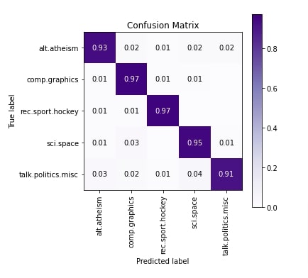
In this section, we have evaluated the performance of the network by calculating accuracy, classification report and confusion matrix metrics. We can notice from the results that the model is doing a pretty good job at predicting the majority of categories. The accuracy of talk.politics.misc is a little less compared to other categories.
We have used various functions available from scikit-learn to calculate metrics. Please feel free to check the below tutorial if you want to know about metrics available from sklearn in detail as the majority of them are covered in it.
Below, we have used scikit-plot Python library to plot the confusion matrix. Please feel free to check the below link if you want to know about it and other ML metric visualizations provided by it.
from sklearn.metrics import accuracy_score, classification_report

train_preds = model.predict(X_train)
test_preds = model.predict(X_test)

print("Train Accuracy : {:.3f}".format(accuracy_score(Y_train, np.argmax(train_preds, axis=1))))
print("Test  Accuracy : {:.3f}".format(accuracy_score(Y_test, np.argmax(test_preds, axis=1))))
print("\nClassification Report : ")
print(classification_report(Y_test, np.argmax(test_preds, axis=1), target_names=selected_categories))
from sklearn.metrics import confusion_matrix
import scikitplot as skplt
import matplotlib.pyplot as plt

skplt.metrics.plot_confusion_matrix([selected_categories[i] for i in Y_test], [selected_categories[i] for i in np.argmax(test_preds, axis=1)],
                                    normalize=True,
                                    title="Confusion Matrix",
                                    cmap="Purples",
                                    hide_zeros=True,
                                    figsize=(5,5)
                                    );
plt.xticks(rotation=90);
5. Explain Model Predictions Using SHAP Partition Explainer 
In this section, we have explained how we can explain predictions made by our model by generating SHAP values using Partition Explainer available from SHAP. Partition Explainer calculates SHAP values by recursively trying a different hierarchy of features of data. We'll try to explain both correct and incorrect predictions made by our model using this explainer.
SHAP library let us generate plots using either its javascript backend or matplotlib. We have used javascript backend as it creates interactive charts that can display values when the mouse is hovered over them as well as let us try a few combinations. In order to use SHAP, we need to initialize it by calling initjs() function on it.
shap.initjs()

We can create a Partition explainer instance using Explainer() constructor available from SHAP. We need to provide is our model, masker, and names of output categories. The masker is needed for text or image data as it'll help us map shap values with tokens of our data (words in our case) and hide parts of data that should not be mapped to any shap values. We can also create Partition explainer using Partition() constructor which has same arguments as Explainer() constructor.
We have created a masker using Text() constructor by providing regular expression pattern 'r"\W+"'. When we provide a regular expression like this, the constructor internally creates a tokenizer using it. We can also create our tokenizer function and provide it to this masker. The tokenizer should return a dictionary with two keys.
- 'input_ids' - The value of this key should be a list of tokens that are not words. It is tokens that are between words like punctuations, spaces, etc. The tokens separate two words.
- 'offset_mapping' - The values of this key should be a list of tuples of length two. These tuples are start and end indexes of tokens available in 'input_ids' values.
When we create a masker using the regular expression 'r"\W+"', it'll internally create a dictionary with the above keys.
Please make a NOTE that even if we don't provide a pattern when creating a masker object, it'll still use the same 'r"\W+"' pattern.
masker = shap.maskers.Text(tokenizer=r"\W+")
explainer = shap.Explainer(model, masker=masker, output_names=selected_categories)

explainer
Visualize SHAP Values For Correct Predictions 
In this section, we have explained a few correct predictions made by our model using SHAP.
We have selected 2 samples from our dataset and printed their contents first. We have printed their contents in tokenized form. Then, we have used our model and made predictions on both samples. We have printed what was actual target category, predicted target category, and probability of predictions.
Then, we have generated the SHAP values of these data samples using Partition explainer. We have called an instance of explainer by providing a list of text samples to it. We'll be generating various visualizations using these generated SHAP values.
In the next cell after it, we have printed the shape of shap values, base values, and data stored inside of shap values object. The base values are values to which shap values are added to generate predictions. As we have two samples and five target categories, the base value shape is (2,5).
import re

X_batch = X_test[3:5]

print("Samples : ")
for text in X_batch:
    print(re.split(r"\W+", text))
    print()

preds_proba = model.predict(X_batch)
preds = preds_proba.argmax(axis=1)

print("Actual    Target Values : {}".format([selected_categories[target] for target in Y_test[3:5]]))
print("Predicted Target Values : {}".format([selected_categories[target] for target in preds]))
print("Predicted Probabilities : {}".format(preds_proba.max(axis=1)))

shap_values = explainer([text.lower() for text in X_batch]) ## Generate SHAP VAlues
print("SHAP Values Shape : {}".format(shap_values.shape))
print("SHAP Base Values  : {}".format(shap_values.base_values))
print("SHAP Data : ")
print(shap_values.data[0])
print(shap_values.data[1])
Text Plots
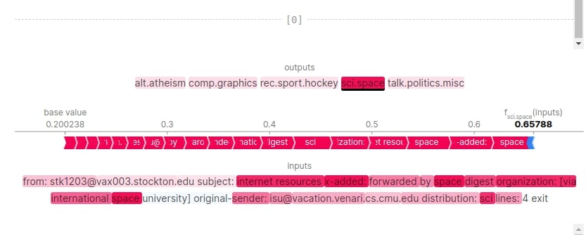
In this section, we have generated a text plot using shap values. We can easily create a text plot by calling text_plot() function of SHAP library and giving it shap values to generate a text plot.
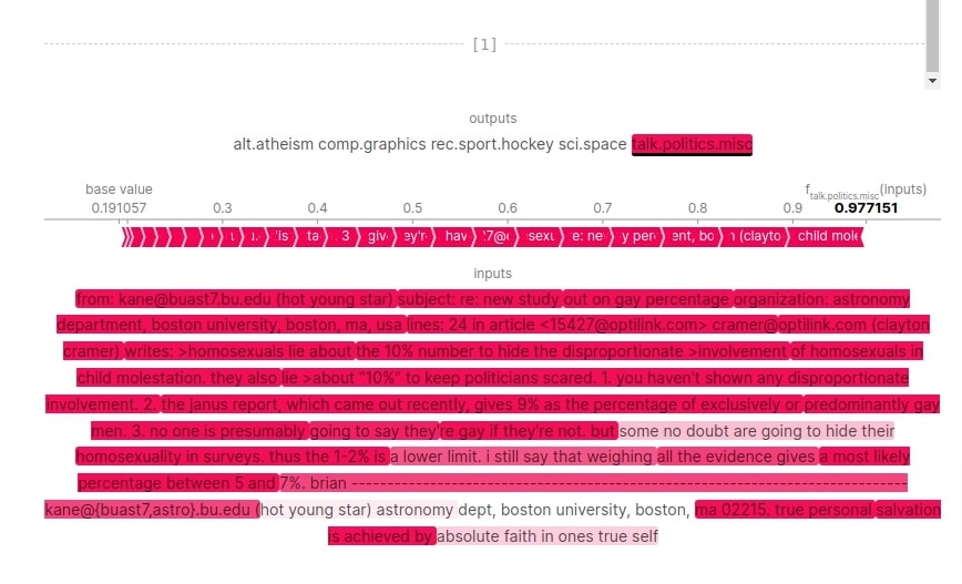
The text plot shows the actual text of the document and shows how much positively or negatively each word contributed to a particular prediction. The chart is interactive where we can click on different output categories and see the results. When we hover over a word, it shows the shap value of that word that contributed to the predictions. The shap values of all words are added to the base value to generate predictions.
In our case, first sample prediction is 'sci.space' with probability 0.657 and second sample prediction is 'talk.politics.misc' with probability of 0.977. These two categories are highlighted with dark colors in the chart. We can click on other categories as well and check their results. The visualizations highlight the words that contributed positively with shades of red color and those contributed negatively with shades of blue color. We can notice from the visualizations how both samples had words that contributed to the prediction category.
shap.text_plot(shap_values)
Bar Charts
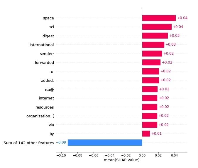
In this section, we have created bar charts that can be analyzed to see which words contributed the most to the prediction.
Below, we have created a first bar chart using average values of 'sci.space' categories. These will help us see which words contributed the most towards that category. We can notice from the results that obvious words like 'space', 'sci', 'international', etc contributed towards that category prediction. We have sorted bars from higher to lower shap values and showed only the most important bars. Please take a look at how we have provided shap values.
shap.plots.bar(shap_values[:,:, selected_categories[preds[0]]].mean(axis=0), max_display=15,
               order=shap.Explanation.argsort.flip)
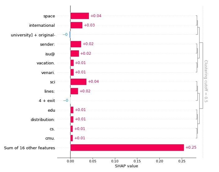
Below, we have created bar charts showing which words and their combinations contributed to predicting category 'sci.space' for 1st sample. It has clustered words that contributed most towards prediction.
shap.plots.bar(shap_values[0,:, selected_categories[preds[0]]], max_display=15,
               order=shap.Explanation.argsort.flip)
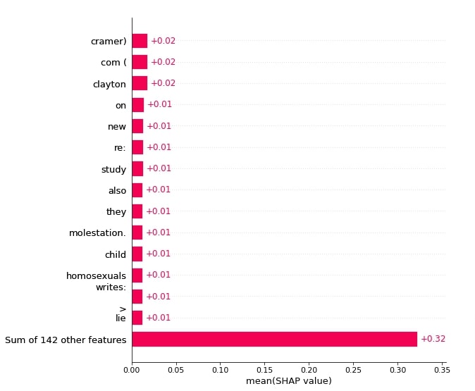
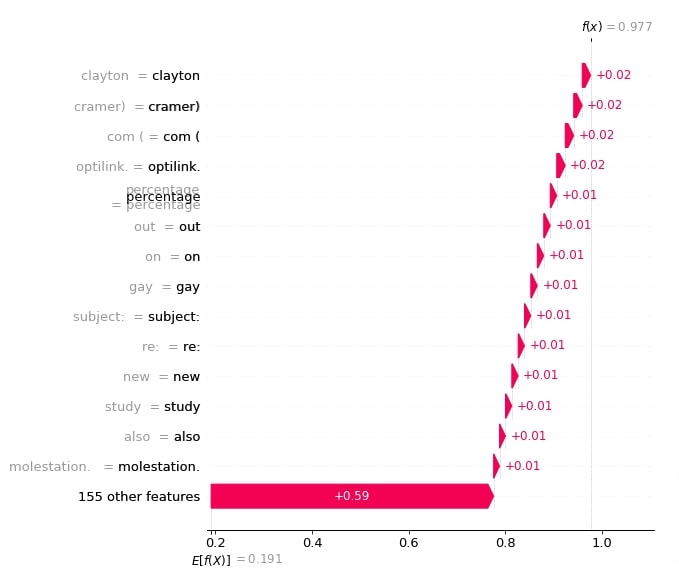
Below, we have created a bar chart showing which words contributed most towards predicting category 'talk.politics.misc'. We can notice that words like 'study', 'molestation', 'homosexuals', etc are contributing more because they can be used by politicians in their speeches and can be topics of common societal problems.
shap.plots.bar(shap_values[:,:, selected_categories[preds[1]]].mean(axis=0), max_display=15,
               order=shap.Explanation.argsort.flip)
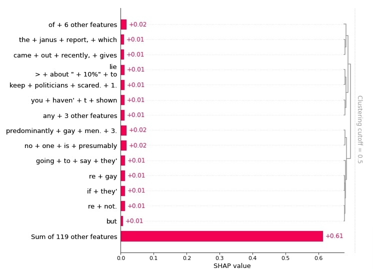
Below, we have created a bar chart showing the combinations of words that contributed to predicting category 'talk.politics.misc' for 2nd samples.
shap.plots.bar(shap_values[1,:, selected_categories[preds[1]]], max_display=15,
               order=shap.Explanation.argsort.flip)
Waterfall Chart
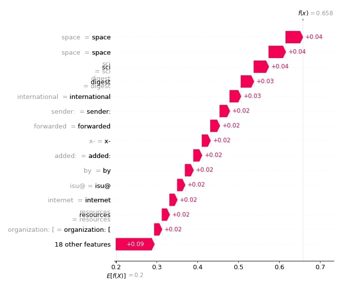
In this section, we have created a waterfall chart that shows how incrementally adding shap values to base value generates the prediction probability.
Below, we have created a waterfall chart for the first sample. It shows how shap values of words contributed to the base value to come to the final prediction probability.
shap.waterfall_plot(shap_values[0][:, selected_categories[preds[0]]], max_display=15)
Below, we have created a waterfall chart for the second sample of data.
shap.waterfall_plot(shap_values[1][:, selected_categories[preds[1]]], max_display=15)
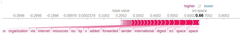
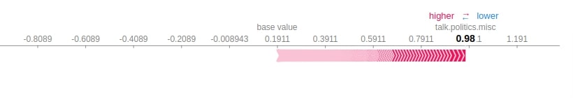
Force Plot
In this section, we have created a force plot that shows shap values in an additive force layout.
print(selected_categories)
Below, we have created a force plot for our 1st sample predictions. In order to create a force plot, we need to provide base values, shap values, and features of data (words in our case). It is an interactive plot that can be used to analyze which words contributed most towards prediction.
import re

tokens = re.split("\W+", X_batch[0].lower())

shap.force_plot(shap_values.base_values[0][preds[0]], shap_values[0][:, preds[0]].values,
                feature_names = tokens[:-1], out_names=selected_categories[preds[0]])
Below, we have created a force plot for 2nd sample.
import re

tokens = re.split("\W+", X_batch[1].lower())

shap.force_plot(shap_values.base_values[1][preds[1]], shap_values[1][:, preds[1]].values,
                feature_names = tokens[:-1], out_names=selected_categories[preds[1]])
Visualize SHAP Values For Incorrect Predictions 
In this section, we have explained the wrong predictions made by our model. We have created various visualizations that show which words contributed to predicting a particular category.
In order to find our wrong predictions, we have first made predictions for all test samples. Then, we have compared them with actual test target values and retrieved indexes of samples that are predicted wrong. We have then used the first two indexes from those wrong predictions indexes for explanation purposes.
We have made predictions using our model for those two samples and printed our prediction categories. We have also printed the original target categories for comparison purposes. Also, we have printed the probabilities with which our model predicted the wrong category (i.e. how sure was our model in predicting it). For first sample actual category was 'sci.space' but our model predicted 'comp.graphics' and for second sample actual category was 'comp.graphics' but our model predicted 'sci.space'.
Then, we have generated shap values using Partition explainer by giving data samples to it.
import re

Y_test_preds = model.predict(X_test)
Y_test_preds = Y_test_preds.argmax(axis=1)

wrong_preds = np.argwhere(Y_test!=Y_test_preds)
X_batch = X_test[wrong_preds.flatten()[:2]]

print("Samples : ")
for text in X_batch:
    print(re.split(r"\W+", text))
    print()

preds_proba = model.predict(X_batch)
preds = preds_proba.argmax(axis=1)

print("Actual    Target Values : {}".format([selected_categories[target] for target in Y_test[wrong_preds.flatten()[:2]]]))
print("Predicted Target Values : {}".format([selected_categories[target] for target in preds]))
print("Predicted Probabilities : {}".format(preds_proba.max(axis=1)))

shap_values = explainer([text.lower() for text in X_batch])

shap_values.shape
print("SHAP Values Shape : {}".format(shap_values.shape))
print("SHAP Base Values  : {}".format(shap_values.base_values))
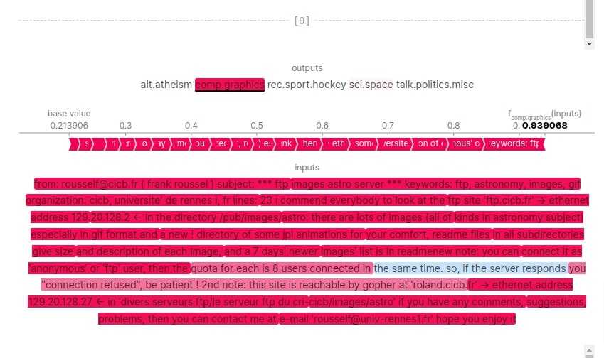
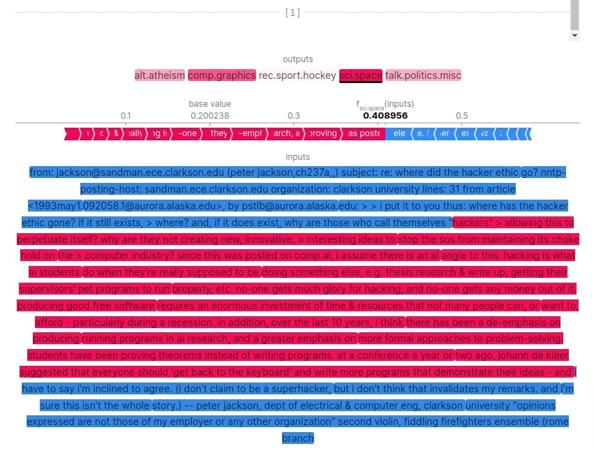
Text Plot
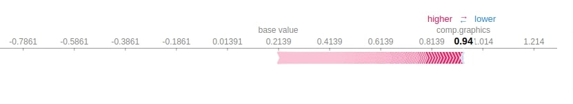
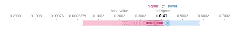
Below, we have plotted a text plot showing which shap values contributed to the prediction category. We can notice from the results that the first samples have words like 'ftp', 'ethernet', 'gif', 'image', 'directory', etc that could have contributed towards predicting sample as 'comp.graphics'. For second sample, the model is not much confident about prediction with probability of 0.40 for 'sci.space' followed by 0.285 for 'comp.graphics'.
shap.text_plot(shap_values)
Bar Charts
In this section, we have created various bar charts showing words that contributed to predictions.
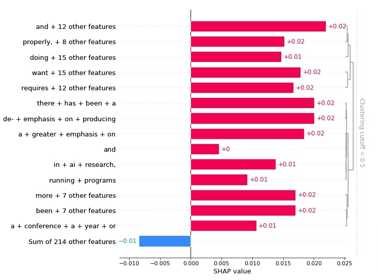
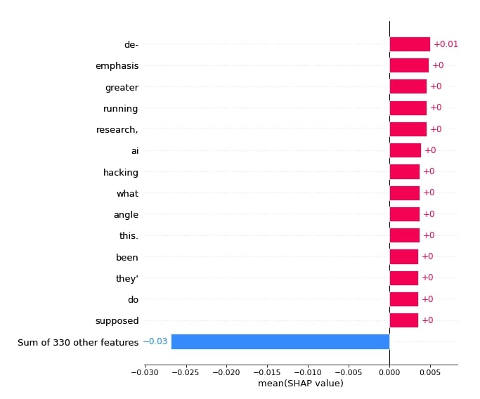
Below, we have created a bar chart showing word combinations that contributed towards predicting category 'comp.graphics' for the first sample.
shap.plots.bar(shap_values[0,:, selected_categories[preds[0]]], max_display=15,
               order=shap.Explanation.argsort.flip)
Below, we have created a bar chart showing words that contributed towards predicting category 'comp.graphics'.
shap.plots.bar(shap_values[:,:, selected_categories[preds[0]]].mean(axis=0), max_display=15,
               order=shap.Explanation.argsort.flip)
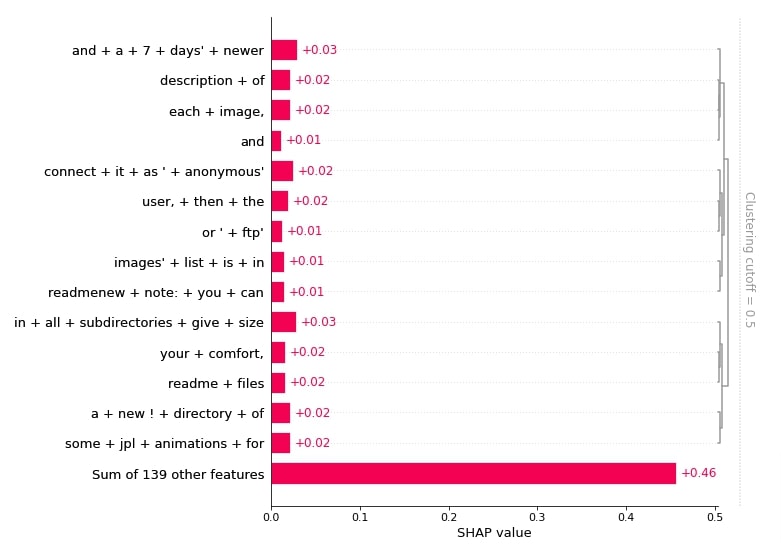
Below, we have created a bar chart showing word combinations that contributed towards predicting category 'sci.space' for the second sample.
shap.plots.bar(shap_values[1,:, selected_categories[preds[1]]], max_display=15,
               order=shap.Explanation.argsort.flip)
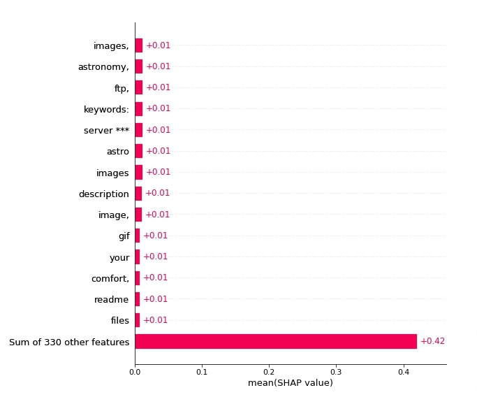
Below, we have created a bar chart showing words that contributed towards predicting category 'sci.space'.
shap.plots.bar(shap_values[:,:, selected_categories[preds[1]]].mean(axis=0), max_display=15,
               order=shap.Explanation.argsort.flip)
Force Plots
In this section, we have created force plots showing words' contribution to prediction according to their shap values. We have created a force plot for both samples one after another.
print(selected_categories)
import re

tokens = re.split("\W+", X_batch[0].lower())

shap.force_plot(shap_values.base_values[0][preds[0]], shap_values[0][:, preds[0]].values,
                feature_names = tokens[:-1], out_names=selected_categories[preds[0]])
import re

tokens = re.split("\W+", X_batch[1].lower())

shap.force_plot(shap_values.base_values[1][preds[1]], shap_values[1][:, preds[1]].values,
                feature_names = tokens[:-1], out_names=selected_categories[preds[1]])
This ends our small tutorial explaining how we can use python library SHAP to explain predictions made by text classification models created using keras. Please feel free to let us know your views in the comments section.
References
 Sunny Solanki
Sunny Solanki
Intro: Software Developer | Youtuber | Bonsai Enthusiast
About: Sunny Solanki holds a bachelor's degree in Information Technology (2006-2010) from L.D. College of Engineering. Post completion of his graduation, he has 8.5+ years of experience (2011-2019) in the IT Industry (TCS). His IT experience involves working on Python & Java Projects with US/Canada banking clients. Since 2020, he’s primarily concentrating on growing CoderzColumn.
His main areas of interest are AI, Machine Learning, Data Visualization, and Concurrent Programming. He has good hands-on with Python and its ecosystem libraries.
Apart from his tech life, he prefers reading biographies and autobiographies. And yes, he spends his leisure time taking care of his plants and a few pre-Bonsai trees.
Contact: sunny.2309@yahoo.in


![YouTube Subscribe]() Comfortable Learning through Video Tutorials?
Comfortable Learning through Video Tutorials?
If you are more comfortable learning through video tutorials then we would recommend that you subscribe to our YouTube channel.
![Need Help]() Stuck Somewhere? Need Help with Coding? Have Doubts About the Topic/Code?
Stuck Somewhere? Need Help with Coding? Have Doubts About the Topic/Code?
 Stuck Somewhere? Need Help with Coding? Have Doubts About the Topic/Code?
When going through coding examples, it's quite common to have doubts and errors.
If you have doubts about some code examples or are stuck somewhere when trying our code, send us an email at coderzcolumn07@gmail.com. We'll help you or point you in the direction where you can find a solution to your problem.
You can even send us a mail if you are trying something new and need guidance regarding coding. We'll try to respond as soon as possible.
![Share Views]() Want to Share Your Views? Have Any Suggestions?
Want to Share Your Views? Have Any Suggestions?
 Want to Share Your Views? Have Any Suggestions?
If you want to
- provide some suggestions on topic
- share your views
- include some details in tutorial
- suggest some new topics on which we should create tutorials/blogs
 shap-values, text-classification, keras