MXNet: LSTM Networks for Time-Series Data (Regression Tasks)
Time-series data as its name says has a time component present in it which is generally referred to as a temporal component. Generally, Time-series data has one or more data variables measured at a specified interval of time. The most common example of time-series data is stock price recorded every minute/hour/day. Time-series data can also have trend and seasonality. When making predictions of any example with time-series data, we generally use one or more previous examples to make predictions. As time-series data have an order, we can not shuffle examples of it and we need to design networks that could capture this order to make better predictions. Various researches have shown that Recurrent Neural Networks (RNNs) and its variant are quite good at capturing sequence order in datasets hence giving better results for tasks involving time-series data compared to other network architectures.
As a part of this tutorial, we have explained how we can create Recurrent Neural Networks (RNNs) consisting of LSTM layers using Python Deep Learning library MXNet for solving time-series regression task. The dataset that we have used in our tutorial is a Tetouan City Power Consumption dataset available from UCI ML Datasets Repository. The dataset is a multivariate dataset and has data variables like temperature, humidity, wind speed, diffuse flows, power consumption, etc measured every 10 minutes. We'll prepare our network to predict the power consumption of the city. As we are predicting continuous variable, it'll be regression task. At the end of the tutorial, we have also given a few suggestions on how we can improve network performance further.
Below, we have listed important sections of the Tutorial to give an overview of the material.
Important Sections Of Tutorials
- Prepare Data
- 1.1 Download Data
- 1.2 Load Data
- 1.3 Reorganize Data for Regression Task
- 1.4 Scale Target Values
- 1.5 Create Datasets and Data Loaders
- Define LSTM Regression Network
- Train Network
- Evaluate Network Performance
- Visualize Predictions
- Further Recommendations
Below, we have imported the necessary Python libraries and printed the versions that we have used in our tutorial.
import mxnet

print("MXNet Version : {}".format(mxnet.__version__))
1. Prepare Data 
In this section, we have organized our data so that it can be given to a neural network for processing. As mentioned earlier, when working with time-series data, in order to make a prediction of current or future values, the best data features to use are that of a few previous examples data features. In our case, we have decided that in order to make a prediction of the current example's target value, we'll look at data features of 30 previous examples. Don't worry if you don't understand what we just said, it'll become pretty clear when we implement them below.
1.1 Download Data
Below, we have downloaded Tetouan City power consumption dataset. The dataset has information about power distribution units from three different electricity distribution networks and a few other data variables for Tetouan city located in Morocco. This is the dataset that we'll use for our task. Next, we'll load it in memory to give an idea about its contents.
!wget https://archive.ics.uci.edu/ml/machine-learning-databases/00616/Tetuan%20City%20power%20consumption.csv
%ls
1.2 Load Data
Below, we have loaded our dataset into the main memory as a pandas dataframe. After loading the dataset, we have set DateTime column as an index of the dataframe. The dataset has the below-mentioned data variables recorded every 10 minutes.
- Date-time
- Temperature
- Humidity
- Wind Speed
- General diffuse flows
- Diffuse flows
- Zone 1 Power Consumption (units)
- Zone 2 Power Consumption
- Zone 3 Power Consumption
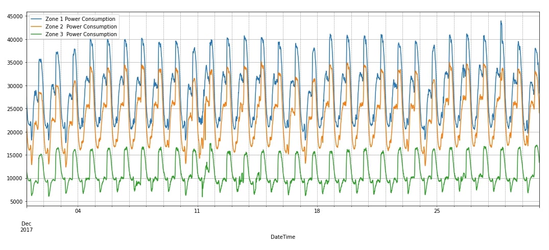
After loading the dataset, we have also displayed the first few columns of the dataset to give an idea about its contents. We can notice from the dataset that power units recorded by three different zones have quite a high range compared to other columns of data.
Apart from displaying data, we have also plotted a line chart showing the power consumption of three zones for December 2017. We can notice from the chart that data has clearly seasonality.
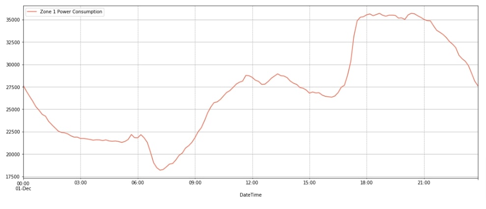
We have also plotted another line chart to show the consumption of units for a single day of Zone 1 to give an idea of how demand varies throughout the day. The demand is low at the beginning of the and then starts rising from 6-7 AM till 12 PM. Then, it stays almost the same till 5-6 PM and then rises again till 9 PM. After 9 PM demands drop till morning.
import pandas as pd

data_df = pd.read_csv("Tetuan City power consumption.csv")
data_df["DateTime"] = pd.to_datetime(data_df["DateTime"])
data_df = data_df.set_index('DateTime')
data_df.columns = [col.strip() for col in data_df.columns]

print("Columns : {}".format(data_df.columns.values.tolist()))
print("Dataset Shape : {}".format(data_df.shape))

data_df.head()
import matplotlib.pyplot as plt

data_df.loc["2017-12"].plot(y=["Zone 1 Power Consumption", "Zone 2  Power Consumption", "Zone 3  Power Consumption"], figsize=(18, 7), grid=True);
plt.grid(which='minor', linestyle=':', linewidth='0.5', color='black');
import matplotlib.pyplot as plt

data_df.loc["2017-12-1"].plot(y="Zone 1 Power Consumption", figsize=(18, 7), color="tomato", grid=True);
plt.grid(which='minor', linestyle=':', linewidth='0.5', color='black');
1.3 Reorganize Data for Regression Task
In this section, we are actually organizing our data to be given to the network. We have decided that data of columns ['Temperature', 'Humidity', 'Wind Speed', 'general diffuse flows', 'diffuse flows'] will be used as data features (X) and data of column Zone 1 Power Consumption will be our target variable (Y).
As discussed earlier, we'll be using data features of 30 previous examples to make a prediction of the target value for the current example. As data is recorded every 10 minutes, the previous 30 examples comprise 5 hours data. So, we'll be looking at data from the previous 5 hours to make the prediction of current. We have declared the variable lookback and set its value to 30.
In order to prepare data, we are moving a window of size lookback through data one step at a time. The examples that fall into the window will be taken as data features and the target value of the example after the window will be our target value. The window will keep moving by one step at a time recording data features (X_organized) and target values (Y_organized). Organizing data in this way will help LSTM layers to capture sequences in data.
Once data is organized as per our need, we divided data into the train (first 50k examples) and test (remaining examples) sets. We have wrapped datasets into mxnet nd arrays as required by MXNet networks. We have also printed the shape of the train and test sets for reference purposes.
import numpy as np
from mxnet import nd

feature_cols = ['Temperature', 'Humidity', 'Wind Speed', 'general diffuse flows', 'diffuse flows']
target_col = 'Zone 1 Power Consumption'

X = data_df[feature_cols].values
Y = data_df[target_col].values

n_features = X.shape[1]
lookback = 30 ## 5 hours lookback to make prediction

X_organized, Y_organized = [], []
for i in range(0, X.shape[0]-lookback, 1):
    X_organized.append(X[i:i+lookback])
    Y_organized.append(Y[i+lookback])

X_organized, Y_organized = np.array(X_organized), np.array(Y_organized)
X_train, Y_train, X_test, Y_test = X_organized[:50000], Y_organized[:50000], X_organized[50000:], Y_organized[50000:]
X_train, X_test = nd.array(X_train, dtype=np.float32),nd.array(X_test, dtype=np.float32)


X_organized.shape, Y_organized.shape, X_train.shape, Y_train.shape, X_test.shape, Y_test.shape
1.4 Scale Target Values
Here, we have normalized the values of our target variable. The reason for doing normalization is that the data of the target variable is in quite a high range compared to other data features columns as we had highlighted earlier. This can make gradient descent optimization algorithm hard to converge. In order to make the task of our optimization algorithm, we have normalized the target variable.
We have first calculated the mean and standard deviation of target values. Then, we subtracted the mean from the train and test target values. After subtracting, we have divided them by standard deviation. We have printed the new range of data as well.
When making predictions for our task, we'll reverse this process to make an actual prediction.
mean, std = Y_train.mean(), Y_train.std()

print("Mean : {:.2f}, Standard Deviation : {:.2f}".format(mean, std))
Y_train_scaled, Y_test_scaled = (Y_train - mean)/std , (Y_test-mean)/std
Y_train_scaled, Y_test_scaled = nd.array(Y_train_scaled, dtype=np.float32),nd.array(Y_test_scaled, dtype=np.float32)

Y_train_scaled.min(), Y_train_scaled.max(), Y_test_scaled.min(), Y_test_scaled.max()
1.5 Create Datasets and Data Loaders
In this section, we have first simply wrapped train and test arrays into ArrayDataset object. Then, we created data loaders from these dataset objects. The data loaders will let us loop through data in batches during the training process. We have set batch size to 128 and shuffle is set to False as we don't want to disturb ordering. We can't shuffle examples because this is time-series data and order is important.
from mxnet.gluon.data import ArrayDataset, DataLoader

train_dataset = ArrayDataset(X_train, Y_train_scaled)
test_dataset  = ArrayDataset(X_test, Y_test_scaled)

train_loader = DataLoader(train_dataset, batch_size=128, shuffle=False)
test_loader  = DataLoader(test_dataset,  batch_size=128, shuffle=False)
for X, Y in train_loader:
    print(X.shape, Y.shape)
    break
2. Define LSTM Regression Network 
In this section, we have defined a simple RNN that we'll use for our regression task. The network consists of two LSTM layers and one dense layer. The first two layers of the network are LSTM layers with 256 output units each. We have stacked two LSTM layers to better capture the order present in time-series data. MXNet provides us with LSTM() constructor through 'gluon.nn' sub-module. It let us stack more than one LSTM layer. We have provided num_layers parameter to 2 informing the constructor to stack two LSTM layers. The output of the second LSTM layer is given to a dense layer that has one output unit. The output of the dense layer is a prediction of our network.
After defining the network, we initialized it and performed a forward pass through it using random data for verification purposes. We have also printed the summary of output shapes of layers and parameters count per layer.
Please make a NOTE that we have not covered the inner workings of LSTM layers here as we have assumed that the reader has little background on them. If you want to learn about it then we recommend that you go through the below link as it'll help you better understand it.
Below, we have included another link for people who are new to MXNet and want to learn how to design networks using it. It can be considered an MXNet starter tutorial.
from mxnet.gluon import nn, rnn

hidden_dim = 256
n_layers = 2

class LSTMRegressor(nn.Block):
    def __init__(self, **kwargs):
        super(LSTMRegressor, self).__init__(**kwargs)
        self.lstm = rnn.LSTM(hidden_size=hidden_dim, num_layers=n_layers, layout="NTC", input_size=n_features)
        self.dense = nn.Dense(1)

    def forward(self, x):
        x = self.lstm(x)

        return self.dense(x[:, -1])

model = LSTMRegressor()

model
from mxnet import init, initializer

model.initialize(initializer.Xavier())
preds = model(nd.random.randn(10,lookback, n_features))

preds.shape
model.summary(nd.random.randn(10,lookback, n_features))
3. Train Network 
In this section, we have trained our network. In order to train it, we have defined a helper function. The function takes Trainer object (network parameters are in it), train data loader, validation data loader, and a number of epochs. The function executes the training loop a number of epochs times. For each epoch, it loops through training data in batches using a train data loader. For each batch, it performs a forward pass to make predictions, calculates loss, calculates gradients, and updates network parameters using gradients. It records the loss of each batch and prints the average loss of all batches at the end of an epoch. There is another helper function that helps us calculates validation loss.
from mxnet import autograd
from tqdm import tqdm
from sklearn.metrics import accuracy_score

def CalcValLoss(model, val_loader):
    losses = []
    for X_batch, Y_batch in val_loader:
        val_loss = loss_func(model(X_batch), Y_batch)
        val_loss = val_loss.mean().asscalar()
        losses.append(val_loss)
    print("Valid Loss : {:.3f}".format(np.array(losses).mean()))

def TrainModelInBatches(trainer, train_loader, val_loader, epochs):
    for i in range(1, epochs+1):
        losses = [] ## Record loss of each batch
        for X_batch, Y_batch in tqdm(train_loader):
            with autograd.record():
                preds = model(X_batch) ## Forward pass to make predictions
                train_loss = loss_func(preds.squeeze(), Y_batch) ## Calculate Loss
            train_loss.backward() ## Calculate Gradients

            train_loss = train_loss.mean().asscalar()
            losses.append(train_loss)

            trainer.step(len(X_batch)) ## Update weights

        print("Train Loss : {:.3f}".format(np.array(losses).mean()))
        CalcValLoss(model, val_loader)
Below, we are actually training our network by calling training routine. We have initialized a number of epochs to 15 and the learning rate to 0.001. Then, we have initialized model, l2 loss (mean squared error loss), Adam optimizer and Trainer object (network parameters). At last, we have called our training function with the necessary parameters to perform training. We can notice from the reducing loss values getting printed after each epoch that our network seems to be doing a good job at the regression task.
from mxnet import gluon, initializer
from mxnet.gluon import loss
from mxnet import autograd
from mxnet import optimizer

epochs=15
learning_rate = 0.001

model = LSTMRegressor()
model.initialize(initializer.Xavier())
loss_func = loss.L2Loss()
optimizer = optimizer.Adam(learning_rate=learning_rate)

trainer = gluon.Trainer(model.collect_params(), optimizer)

TrainModelInBatches(trainer, train_loader, test_loader, epochs)
4. Evaluate Network Performance 
In this section, we are evaluating the performance of our trained network on test data.
Below, we have first made predictions on the test dataset using our trained network. Then, we have de-normalized predictions using the training mean and standard deviation that we had calculated earlier. This will bring predictions into the actual range.
Then, in the next cell, we have calculated metrics 'mean squared error (MSE)','r2 score' and 'mean absolute error (MAE)' on test predictions. R2 score is a very commonly used metric to check the performance of the model on regression tasks. We have calculated score using r2_score function available from scikit-learn. It returns values in the range 0-1 and values near 1 are considered signs of a good generalized model. We can notice from our score that our model is doing a good job at the task.
If you want to know how r2 score works internally then we would suggest the below link. It explains the majority of metrics available from sklearn in-depth.
test_preds = model(X_test) ## Make Predictions on test dataset
test_preds  = (test_preds*std) + mean ## Upscaling Predictions

test_preds[:5]
from sklearn.metrics import r2_score, mean_squared_error, mean_absolute_error

print("Test  MSE : {:.2f}".format(mean_squared_error(test_preds.asnumpy().squeeze(), Y_test)))
print("Test  R^2 Score : {:.2f}".format(r2_score(test_preds.asnumpy().squeeze(), Y_test)))
print("Test  MAE : {:.2f}".format(mean_absolute_error(test_preds.asnumpy().squeeze(), Y_test)))
5. Visualize Predictions 
In this section, we are visualizing predictions next to actual values to have an even deeper look at the performance of our network.
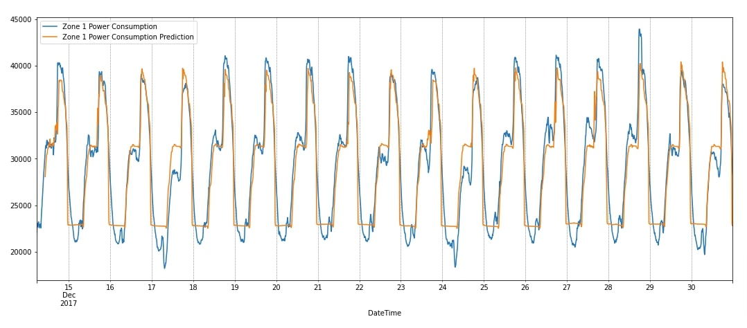
Below, we have first added test predictions to our dataframe. Then, we visualized the original zone 1 consumption units and predicted units as a line chart. We can notice from the chart that our model is better at capturing peaks compared to downward movements. Overall, it has done a good job at capturing the seasonality. We can still improve the model by trying a few suggestions we have given next.
data_df_final = data_df[50000:].copy()

data_df_final["Zone 1 Power Consumption Prediction"] = [None]*lookback + test_preds.asnumpy().squeeze().tolist()

data_df_final.tail()
data_df_final.plot(y=["Zone 1 Power Consumption", "Zone 1 Power Consumption Prediction"],figsize=(18,7));
plt.grid(which='minor', linestyle=':', linewidth='0.5', color='black');
6. Further Recommendations 
- Train the network for more epochs to see whether it is improving further.
- Try different output units for LSTM layers.
- Stack more LSTM layers. This can increase training time hence think twice.
- Try adding more dense layers after LSTM layers.
- Try adding dropout.
- Try different activation functions.
- Create network architecture that predicts more than one future value. Our network predicts only a single future value. You can design a network that can predict 5-10 or more days. You need to organize data also to make more than one future prediction.
- Add datetime-related features like day, day of the week, month, hour, AM/PM, month start, month-end, quarter start, quarter-end, year start, year-end, etc.
- Try learning rate schedulers during training.
 Sunny Solanki
Sunny Solanki
Intro: Software Developer | Youtuber | Bonsai Enthusiast
About: Sunny Solanki holds a bachelor's degree in Information Technology (2006-2010) from L.D. College of Engineering. Post completion of his graduation, he has 8.5+ years of experience (2011-2019) in the IT Industry (TCS). His IT experience involves working on Python & Java Projects with US/Canada banking clients. Since 2020, he’s primarily concentrating on growing CoderzColumn.
His main areas of interest are AI, Machine Learning, Data Visualization, and Concurrent Programming. He has good hands-on with Python and its ecosystem libraries.
Apart from his tech life, he prefers reading biographies and autobiographies. And yes, he spends his leisure time taking care of his plants and a few pre-Bonsai trees.
Contact: sunny.2309@yahoo.in


![YouTube Subscribe]() Comfortable Learning through Video Tutorials?
Comfortable Learning through Video Tutorials?
If you are more comfortable learning through video tutorials then we would recommend that you subscribe to our YouTube channel.
![Need Help]() Stuck Somewhere? Need Help with Coding? Have Doubts About the Topic/Code?
Stuck Somewhere? Need Help with Coding? Have Doubts About the Topic/Code?
 Stuck Somewhere? Need Help with Coding? Have Doubts About the Topic/Code?
When going through coding examples, it's quite common to have doubts and errors.
If you have doubts about some code examples or are stuck somewhere when trying our code, send us an email at coderzcolumn07@gmail.com. We'll help you or point you in the direction where you can find a solution to your problem.
You can even send us a mail if you are trying something new and need guidance regarding coding. We'll try to respond as soon as possible.
![Share Views]() Want to Share Your Views? Have Any Suggestions?
Want to Share Your Views? Have Any Suggestions?
 Want to Share Your Views? Have Any Suggestions?
If you want to
- provide some suggestions on topic
- share your views
- include some details in tutorial
- suggest some new topics on which we should create tutorials/blogs
 mxnet, time-series, lstm, regression