Text Classification Using Keras Networks
Text classification is a task of natural language processing where we classify text documents into categories. There are various ways to classify documents. In order to classify documents using Machine learning algorithms, we need to convert them from text to a list of floats. There are different approaches to turn a text document into a list of floats like we can calculate the frequency of words, frequency of characters, term frequency-inverse document frequency (Tf-IDF) of words/characters, embeddings for words, etc. Once text data is converted to a list of floats, we can feed them to different ML algorithms to make predictions.
As a part of this tutorial, we'll be using keras networks to classify text documents. We have used 20 newsgroups dataset available from scikit-learn for our task. We'll try word frequency and Tf-Idf approaches as a part of the tutorial. If the reader is interested in learning about how word frequency and Tf-Idf approaches work then please feel free to check the below tutorial that discusses it in detail with examples.
Below, we have listed important sections of tutorial to give an overview of the material covered.
Important Sections Of Tutorial
- Load Data
- Word Frequency Text Vectorization
- 1.1 Vectorize Text Data
- 1.2 Create Neural Network
- 1.3 Compile And Train Network
- 1.4 Evaluate Model Performance
- Tf-Idf Text Vectorization
- Multi-Hot Text Vectorization
- Tf-Idf + (1,3) Ngrams Text Vectorization
- Scikit-Learn Tf-Idf Vectorizer
- Other Approaches to Try
Below, we have loaded the keras library and printed the version of it that we have used in our tutorial.
import tensorflow
from tensorflow import keras

print("Keras Version : {}".format(keras.__version__))
Load Data 
In this section, we have loaded 20 newsgroups dataset available from scikit-learn. The dataset has 18k new posts about 20 different topics. As a part of this tutorial, we have considered only 5 categories hence we have loaded posts from these 5 categories. We have listed down all 20 different topics first. Then select 5 categories for which to load data. The scikit-learn provides function named fetch_20newsgroups() from datasets sub-module to load data. The data is already divided into train and test sets. We need to provide which dataset (train/test) we need to load to the function.
import numpy as np
from sklearn import datasets
import gc

all_categories = ['alt.atheism','comp.graphics','comp.os.ms-windows.misc','comp.sys.ibm.pc.hardware',
                  'comp.sys.mac.hardware','comp.windows.x', 'misc.forsale','rec.autos','rec.motorcycles',
                  'rec.sport.baseball','rec.sport.hockey','sci.crypt','sci.electronics','sci.med',
                  'sci.space','soc.religion.christian','talk.politics.guns','talk.politics.mideast',
                  'talk.politics.misc','talk.religion.misc']

selected_categories = ['alt.atheism','comp.graphics','rec.sport.hockey','sci.space','talk.politics.misc']

X_train, Y_train = datasets.fetch_20newsgroups(subset="train", categories=selected_categories, return_X_y=True)
X_test , Y_test  = datasets.fetch_20newsgroups(subset="test", categories=selected_categories, return_X_y=True)

X_train = np.array(X_train)
X_test = np.array(X_test)

classes = np.unique(Y_train)
mapping = dict(zip(classes, selected_categories))

len(X_train), len(X_test), classes, mapping
1. Word Frequency Text Vectorization 
In this section, we are vectorizing text data to float where floats represent the frequency of words in an individual sample. We need to convert text data to floats as our network works on floats. We have then trained the network on the dataset of the frequency of words. Keras provides us with preprocessing layer named TextVectorization that we can use to convert text data to floats.
1.1 Vectorize Text Data
In this section, we have adapted our TextVectorization layer to our dataset. In order to use TextVectorization layer in our network, we first need to adapt it by giving our data first so that it can populate the vocabulary using which it'll convert text data to a list of floats. The vocabulary generally has unique words that appeared across all documents/samples of our data. There are different approaches to convert text to a list of floats which we have covered in different sections. Here, we have asked our text vectorization layer to convert text to a list of floats where floats will be the frequency of words in the document.
After the vectorization layer is adapted and its vocabulary of words is populated, when we convert a text document to a list of floats, it'll have the same length as the length of our vocabulary. The words that appear in our document will have a frequency of that word in our document present at the index of that word in the dictionary. This will become more clear when we explain with an example below.
We can create text vectorization layer using TextVectorization() constructor. It has a list of important parameters that can be helpful to try different approaches for converting text to floats.
- max_tokens - It accepts integer values specifying the maximum size of the vocabulary. If we have many documents then this vocabulary of words can become huge. We can limit the vocab size by setting this parameter.
- standardize - It accepts one of the below options specifying any standard preprocessing to perform on text.
- None - No preprocessing.
- 'lower_and_strip_punctuation' - First lowercase text and then remove punctuations.
- 'lower' - Lowercase text.
- 'strip_punctuation' - Remove punctuations.
- split - This parameter is responsible to convert a text document to a list of tokens (words/characters). It accepts a list of options.
- None - Do not split input data. This option is used when we are giving a list of words/characters as input to layer instead of the whole text of a document.
- 'whitespace' - It splits text on whitespace.
- 'character' - It splits text into a list of characters.
- callable - We can also provide a function to this parameter that takes a text of the document as input and returns a list of tokens.
- output_mode - This option specifies output type of list of floats.
- 'int' - It returns indexes of words in the document in the list of floats at word location in vocabulary.
- 'count' - It returns word frequency in the list of floats at word location in vocabulary.
- 'tf_idf' -It returns TF-IDF (Term Frequency-Inverse Document Frequency) values of words.
- 'multi_hot' - It returns 1 if a word is present in doc else 0 in the list of words at word location in vocabulary.
- ngrams - This accepts integer or tuple of integers specifying n-grams to use. If a single integer is specified then n-grams according to that integer is used. If a tuple is specified then all n-grams between and including start and end values are included.
- pad_to_max_tokens - This parameter accepts boolean value specifying whether to pad zeros at the end if length of vocabulary is less than max_tokens.
- vocabulary - We can provide our own vocabulary if we have already calculated one on data. If we provide vocabulary then we don't need to adapt layer to data. Because we had mentioned earlier that we adapt layer to populate vocabulary and if we are providing one already then we don't need to adapt layer. We can directly use it in our network.
Below, we have initialized TextVectorization layer that converts text to a list of floats where floats are the frequency of words present in the document.
text_vectorizer = keras.layers.TextVectorization(max_tokens=None, standardize="lower_and_strip_punctuation",
                                                 split="whitespace", output_mode="count")

text_vectorizer
Below, we have adapted our layer by calling adapt() function. We have given train data to it so that it'll populate a dictionary from it.
text_vectorizer.adapt(X_train, batch_size=512)

gc.collect()
Below, we have retrieved the dictionary from the layer and printed the first few tokens from it. We can notice that it has a list of words. We have also printed dictionary size which is ~47k words in our case. We have then converted the first few samples of our train data to a list of floats.
We can notice from the list of floats that they are the frequency of words. The word 'the' appears 6 times in the first doc, 15 times in the second, and so on. Same way word 'to' appears 2 times in the first doc, 11 times in the second, and so on.
All the words for which it can't find mapping in the dictionary will be mapped to the 0th token named '[UNK]'.
vocab = text_vectorizer.get_vocabulary()
print("Vocab : {}".format(vocab[:10]))
print("Vocab Size : {}".format(text_vectorizer.vocabulary_size()))

out = text_vectorizer(X_train[:5])
print("Output Shape : {}".format(out.shape))

out
Below, we have again initialized our text vectorization layer. This time we have put a limit on the max token at 50k and asked to pad zeros if vocabulary size is zero. Apart from this, we have also adapted the layer using train and test samples both as if we don't include test samples and it has some important words for which layer can't find an entry in vocab then it'll map them to '[UNK]'. This can impact the accuracy of the model on the test dataset.
text_vectorizer = keras.layers.TextVectorization(max_tokens=50000, standardize="lower_and_strip_punctuation",
                                                 split="whitespace", output_mode="count", pad_to_max_tokens=True)

text_vectorizer.adapt(np.concatenate((X_train, X_test)), batch_size=512)

vocab = text_vectorizer.get_vocabulary()
print("Vocab : {}".format(vocab[:10]))
print("Vocab Size : {}".format(text_vectorizer.vocabulary_size()))
out = text_vectorizer(X_train[:5])
print("Output Shape : {}".format(out.shape))
1.2 Create Neural Network
In this section, we have created a function that will initialize our neural network. The function takes as input a trained text vectorizer and creates a network using it as the first layer. Our network consists of four layers of which the first is the text vectorization layer which is the trained TextVectorization layer we created earlier. The next three layers after the text vectorization layer are dense layers with a number of units 128, 64, and 5 (number of classes). The first two dense layers have relu (rectified linear unit) as activation function and the last layer has softmax activation. We'll use this function to initialize the network each time we try a new approach of text vectorization.
After defining a function, we have initialized the network to use for this section.
from tensorflow.keras.models import Sequential
from tensorflow.keras import layers

def create_model(text_vectorizer):
    return Sequential([
                        layers.Input(shape=(1,), dtype="string"),
                        text_vectorizer,
                        #layers.Dense(256, activation="relu"),
                        layers.Dense(128, activation="relu"),
                        layers.Dense(64, activation="relu"),
                        layers.Dense(len(classes), activation="softmax"),
                    ])

model = create_model(text_vectorizer)

model.summary()
1.3 Compile And Train Network
In this section, we have compiled our network to use Adam optimizer, cross entropy loss, and accuracy as metrics. After compiling the network, we have trained the network by providing train and validation data for 10 epochs with a batch size of 256. We can notice from the results that the network is giving good accuracy after 10 epochs of training.
model.compile("adam", "sparse_categorical_crossentropy", metrics=["accuracy"])
history = model.fit(X_train, Y_train, batch_size=256, epochs=10, validation_data=(X_test, Y_test))
gc.collect()
1.4 Evaluate Model Performance
In this section, we have evaluated the performance of our trained model by calculating various metrics. We have first made predictions for the train and test dataset. Then, we have calculated the accuracy of train and test predictions.
Followed by it, we have also calculated the classification report of test prediction which has precision, recall, and f1-score for each target class of data. We can notice from the results that the model is doing good for the majority of the classes. It's little lacking for 'talk.politics.misc' and 'alt.atheism' classes.
If you want to learn about various ML metrics available through scikit-learn then please check the below link which covers the majority of them in detail.
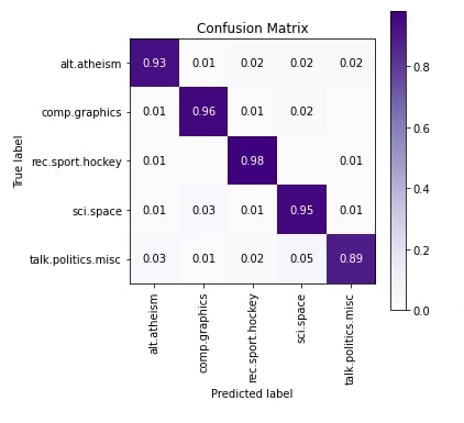
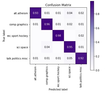
In the cell below, we have plotted the confusion matrix of test predictions. We can notice from the results that a few samples of 'sci.space' and 'comp.graphics' are confused with each other. Few samples of 'talk.politics.misc' are confused with category 'alt.atheism'.
To create confusion matrix visualization, we have used scikit-plot python library. Please feel free to check the below link if you want to learn about it as it has visualizations for many ML metrics.
from sklearn.metrics import accuracy_score, classification_report

train_preds = model.predict(X_train)
test_preds = model.predict(X_test)

print("Train Accuracy : {}".format(accuracy_score(Y_train, np.argmax(train_preds, axis=1))))
print("Test  Accuracy : {}".format(accuracy_score(Y_test, np.argmax(test_preds, axis=1))))
print("\nClassification Report : ")
print(classification_report(Y_test, np.argmax(test_preds, axis=1), target_names=selected_categories))
from sklearn.metrics import confusion_matrix
import scikitplot as skplt
import matplotlib.pyplot as plt

skplt.metrics.plot_confusion_matrix([selected_categories[i] for i in Y_test],
                                    [selected_categories[i] for i in np.argmax(test_preds, axis=1)],
                                    normalize=True,
                                    title="Confusion Matrix",
                                    cmap="Purples",
                                    hide_zeros=True,
                                    figsize=(5,5)
                                    );
plt.xticks(rotation=90);
2. Tf-Idf Text Vectorization 
In this section, we have used Tf-IDF (Term Frequency - Inverse Document Frequency) approach of text vectorization. The majority of the code of this section is almost the same as the previous section with only a change in the text vectorization method. The key idea behind Tf-Idf vectorization is that it generates floats for each word that down-weight the words which appear in the majority of documents giving high importance to words unique per document. This will result in giving less importance to commonly appearing words like 'the', 'a', 'an', 'and', etc.
If you want to understand Tf-Idf in-depth then we recommend that you go through the below link which explains how to work internally.
2.1 Vectorize Text Data And Train Model
In this section, we have first initialized the text vectorization layer with Tf-Idf approach. Then, we have trained it with train and test data to populate its vocabulary.
Then, we have created our neural network using this vectorizer, compiled it, and trained it for 10 epochs. We can notice from the results that it has the almost same result as the word frequency approach earlier.
text_vectorizer = keras.layers.TextVectorization(max_tokens=50000, standardize="lower_and_strip_punctuation",
                                                 split="whitespace", output_mode="tf_idf", pad_to_max_tokens=True)

text_vectorizer.adapt(np.concatenate((X_train, X_test)), batch_size=512)
gc.collect()

model = create_model(text_vectorizer)
model.compile("adam", "sparse_categorical_crossentropy", metrics=["accuracy"])
history = model.fit(X_train, Y_train, batch_size=256, epochs=10, validation_data=(X_test, Y_test))
gc.collect()
2.2 Evaluate Model Performance
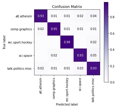
In this section, we have evaluated the performance of the network just like earlier by calculating accuracy, classification report, and confusion matrix. We can notice from the results that 'talk.politics.misc' is doing a little better compared to our previous section results. Surprisingly, some of the 'talk.politics.misc' and 'sci.space' samples are confused with 'talk.politics.misc' as per last column of confusion matrix.
from sklearn.metrics import accuracy_score, classification_report

train_preds = model.predict(X_train)
test_preds = model.predict(X_test)

print("Train Accuracy : {}".format(accuracy_score(Y_train, np.argmax(train_preds, axis=1))))
print("Test  Accuracy : {}".format(accuracy_score(Y_test, np.argmax(test_preds, axis=1))))
print("\nClassification Report : ")
print(classification_report(Y_test, np.argmax(test_preds, axis=1), target_names=selected_categories))
from sklearn.metrics import confusion_matrix
import scikitplot as skplt
import matplotlib.pyplot as plt

skplt.metrics.plot_confusion_matrix([selected_categories[i] for i in Y_test],
                                    [selected_categories[i] for i in np.argmax(test_preds, axis=1)],
                                    normalize=True,
                                    title="Confusion Matrix",
                                    cmap="Purples",
                                    hide_zeros=True,
                                    figsize=(5,5)
                                    );
plt.xticks(rotation=90);
3. Multi-Hot Text Vectorization 
In this section, we have tried another text vectorization approach called multi-hot. This approach is pretty simple as it creates a list of floats which will have 1 or 0 depending on the presence or absence of words in a text document. The majority of the code of this section is the same as a previous section with only a difference in text vectorization approach.
3.1 Vectorize Text Data And Train Model
Below, we have first created a text vectorization layer with 'multi_hot' approach and trained it with data to populate its dictionary. Then, we have created a neural network using this vectorizer, compiled it, and trained it for 10 epochs. We can notice from the validation accuracy that it's a little lower compared to the previous two sections.
text_vectorizer = keras.layers.TextVectorization(max_tokens=50000, standardize="lower_and_strip_punctuation",
                                                 split="whitespace", output_mode="multi_hot",
                                                 pad_to_max_tokens=True)

text_vectorizer.adapt(np.concatenate((X_train, X_test)), batch_size=512)
gc.collect()

model = create_model(text_vectorizer)
model.compile("adam", "sparse_categorical_crossentropy", metrics=["accuracy"])
history = model.fit(X_train, Y_train, batch_size=256, epochs=10, validation_data=(X_test, Y_test))
gc.collect()
3.2 Evaluate Model Performance
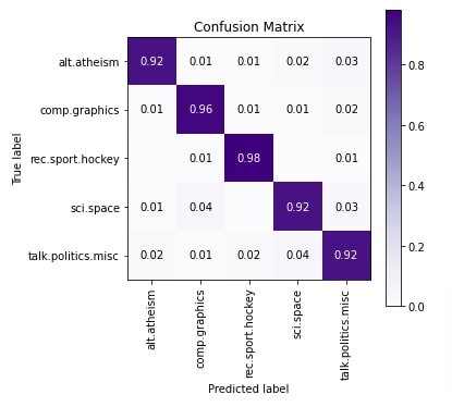
In this section, we have evaluated the performance of network by calculating accuracy, classification report and confusion matrix metrics. We can notice from the results of classification metrics that model is doing okay job for categories 'alt.atheism', 'sci.space' and 'talk.politics.misc'. According to confusion matrix 'talk.politics.misc' category samples are confused with 'sci.space', 'alt.atheism' with 'talk.politics.misc' and 'sci.space' with 'comp.graphics'.
from sklearn.metrics import accuracy_score, classification_report

train_preds = model.predict(X_train)
test_preds = model.predict(X_test)

print("Train Accuracy : {}".format(accuracy_score(Y_train, np.argmax(train_preds, axis=1))))
print("Test  Accuracy : {}".format(accuracy_score(Y_test, np.argmax(test_preds, axis=1))))
print("\nClassification Report : ")
print(classification_report(Y_test, np.argmax(test_preds, axis=1), target_names=selected_categories))
from sklearn.metrics import confusion_matrix
import scikitplot as skplt
import matplotlib.pyplot as plt

skplt.metrics.plot_confusion_matrix([selected_categories[i] for i in Y_test],
                                    [selected_categories[i] for i in np.argmax(test_preds, axis=1)],
                                    normalize=True,
                                    title="Confusion Matrix",
                                    cmap="Purples",
                                    hide_zeros=True,
                                    figsize=(5,5)
                                    );
plt.xticks(rotation=90);
4. Tf-Idf + (1,3) N-grams Text Vectorization 
In this section, we have vectorized our data again using Tf-Idf vectorization but we have used a combination of words along with single words. Till now, all our approaches just used single words which are generally referred to as 1-gram. We can also use all 2-word combinations and 3-word combinations which are referred to as 2-grams and 3-grams respectively. In this approach, we have used 1-gram, 2-grams, and 3-grams with Tf-Idf vectorization. The majority of the code is almost the same as the previous sections as usual.
4.1 Vectorize Text Data And Train Model
Below, we have first created a text vectorizer with Tf-Idf vectorization and (1,3) n-grams. Then, we have trained this vectorizer using our train and test datasets to populate its vocabulary.
Then, we have created our neural network using a trained text vectorizer, compiled it, and trained it for 10 epochs. We can notice from the results that the accuracy is the lowest of all approaches we have tried till now though.
text_vectorizer = keras.layers.TextVectorization(max_tokens=50000, standardize="lower_and_strip_punctuation",
                                                 split="whitespace",
                                                 ngrams=(1,3),
                                                 output_mode="tf_idf", pad_to_max_tokens=True)

text_vectorizer.adapt(np.concatenate((X_train, X_test)), batch_size=512)
gc.collect()

model = create_model(text_vectorizer)
model.compile("adam", "sparse_categorical_crossentropy", metrics=["accuracy"])
history = model.fit(X_train, Y_train, batch_size=256, epochs=10, validation_data=(X_test, Y_test))
gc.collect()
4.2 Evaluate Model Performance
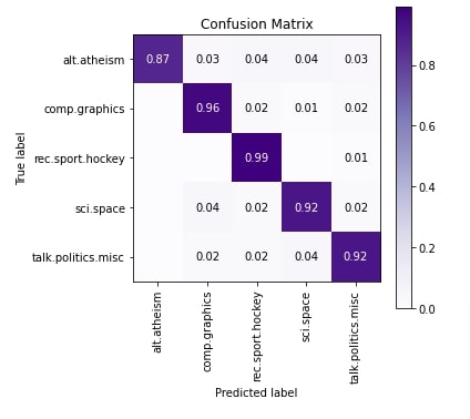
In this section, we have evaluated the performance of the network by calculating accuracy, classification report, and confusion matrix metrics. We can notice from the results that the model is doing an okay job for 'alt.atheism' category as per the classification report. As per the confusion matrix plot, 'alt.atheism' samples are confused with all other categories. The accuracy of 'talk.politics.misc' and 'sci.space' categories is also kind of okay, not best.
from sklearn.metrics import accuracy_score, classification_report

train_preds = model.predict(X_train)
test_preds = model.predict(X_test)

print("Train Accuracy : {}".format(accuracy_score(Y_train, np.argmax(train_preds, axis=1))))
print("Test  Accuracy : {}".format(accuracy_score(Y_test, np.argmax(test_preds, axis=1))))
print("\nClassification Report : ")
print(classification_report(Y_test, np.argmax(test_preds, axis=1), target_names=selected_categories))
from sklearn.metrics import confusion_matrix
import scikitplot as skplt
import matplotlib.pyplot as plt

skplt.metrics.plot_confusion_matrix([selected_categories[i] for i in Y_test],
                                    [selected_categories[i] for i in np.argmax(test_preds, axis=1)],
                                    normalize=True,
                                    title="Confusion Matrix",
                                    cmap="Purples",
                                    hide_zeros=True,
                                    figsize=(5,5)
                                    );
plt.xticks(rotation=90);
5. Scikit-Learn Tf-Idf Vectorizer 
In this section, we have again tried Tf-Idf vectorization on text data but this time we have used TfidfVectorizer available from scikit-learn. We first vectorize data using this vectorizer and then train a neural network on transformed data, unlike our previous approaches where vectorization used to happen inside of network using vectorization layer as the first layer.
5.1 Vectorize Text Data
In this section, we have initialized TfidfVectorizer and trained it with train and test data. We have then vectorized train and test datasets using this trained vectorizer.
from sklearn.feature_extraction.text import TfidfVectorizer, CountVectorizer

vectorizer = TfidfVectorizer(max_features=50000)
vectorizer.fit(np.concatenate((X_train, Y_train)))
X_train_vect = vectorizer.transform(X_train)
X_test_vect = vectorizer.transform(X_test)

X_train_vect, X_test_vect = X_train_vect.toarray(), X_test_vect.toarray()

X_train_vect.shape, X_test_vect.shape
5.2 Create Network
In this section, we have created a neural network that we'll use in this section. The network has the same structure as our previous network with the only difference that we have removed the vectorization layer because we have already performed vectorization earlier and we'll be providing vectorized data to it.
from tensorflow.keras.models import Sequential
from tensorflow.keras import layers

model =  Sequential([
                        layers.Input(shape=X_train_vect.shape[1:]),
                        layers.Dense(128, activation="relu"),
                        layers.Dense(64, activation="relu"),
                        layers.Dense(len(classes), activation="softmax"),
                    ])

model.summary()
5.3 Compile And Train Model
In this section, we have compiled our network and trained it for 10 epochs. We can notice from the results that this network seems to have done the best job as a task with the highest validation accuracy.
model.compile("adam", "sparse_categorical_crossentropy", metrics=["accuracy"])

history = model.fit(X_train_vect, Y_train, batch_size=256, epochs=10, validation_data=(X_test_vect, Y_test))
5.4 Evaluate Model Performance
In this section, we have evaluated the model performance by calculating accuracy, classification report, and confusion matrix metrics. We can notice from the results that the model is doing a good job for the majority of categories. The 'talk.politics.misc' category has a little less accuracy compared to others. Some of the 'alt.atheism' and 'talk.politics.misc' samples are confused with 'sci.space' and some 'sci.space' samples are confused with 'comp.graphics' as per confusion matrix plot.
from sklearn.metrics import accuracy_score, classification_report

train_preds = model.predict(X_train_vect)
test_preds = model.predict(X_test_vect)

print("Train Accuracy : {}".format(accuracy_score(Y_train, np.argmax(train_preds, axis=1))))
print("Test  Accuracy : {}".format(accuracy_score(Y_test, np.argmax(test_preds, axis=1))))
print("\nClassification Report : ")
print(classification_report(Y_test, np.argmax(test_preds, axis=1), target_names=selected_categories))
from sklearn.metrics import confusion_matrix
import scikitplot as skplt
import matplotlib.pyplot as plt

skplt.metrics.plot_confusion_matrix([selected_categories[i] for i in Y_test],
                                    [selected_categories[i] for i in np.argmax(test_preds, axis=1)],
                                    normalize=True,
                                    title="Confusion Matrix",
                                    cmap="Purples",
                                    hide_zeros=True,
                                    figsize=(5,5)
                                    );
plt.xticks(rotation=90);
6. Other Approaches to Try 
- Remove stop words from data and try with TF-IDF, word frequency, and multi-hot approaches.
- Try different vocabulary sizes.
- Try different neural network architectures.
- Try different n-grams with word frequency and multi-hot.
- Create your own tokenizer to tokenize text document to list of words.
- Provide your own dictionary to text vectorization layer, the one created using your tokenizer.
- Keep punctuations and see if it helps improve accuracy.
- Keep uppercase letters as uppercase and check whether it helps improve accuracy.
- Try using character vectorization instead of word vectorization to see if it helps.
This ends our small tutorial explaining how we can perform text classification using deep neural networks. We explained how to solve text classification tasks using keras networks. Please feel free to let us know your views in the comments section.
References
 Sunny Solanki
Sunny Solanki
Intro: Software Developer | Youtuber | Bonsai Enthusiast
About: Sunny Solanki holds a bachelor's degree in Information Technology (2006-2010) from L.D. College of Engineering. Post completion of his graduation, he has 8.5+ years of experience (2011-2019) in the IT Industry (TCS). His IT experience involves working on Python & Java Projects with US/Canada banking clients. Since 2020, he’s primarily concentrating on growing CoderzColumn.
His main areas of interest are AI, Machine Learning, Data Visualization, and Concurrent Programming. He has good hands-on with Python and its ecosystem libraries.
Apart from his tech life, he prefers reading biographies and autobiographies. And yes, he spends his leisure time taking care of his plants and a few pre-Bonsai trees.
Contact: sunny.2309@yahoo.in


![YouTube Subscribe]() Comfortable Learning through Video Tutorials?
Comfortable Learning through Video Tutorials?
If you are more comfortable learning through video tutorials then we would recommend that you subscribe to our YouTube channel.
![Need Help]() Stuck Somewhere? Need Help with Coding? Have Doubts About the Topic/Code?
Stuck Somewhere? Need Help with Coding? Have Doubts About the Topic/Code?
 Stuck Somewhere? Need Help with Coding? Have Doubts About the Topic/Code?
When going through coding examples, it's quite common to have doubts and errors.
If you have doubts about some code examples or are stuck somewhere when trying our code, send us an email at coderzcolumn07@gmail.com. We'll help you or point you in the direction where you can find a solution to your problem.
You can even send us a mail if you are trying something new and need guidance regarding coding. We'll try to respond as soon as possible.
![Share Views]() Want to Share Your Views? Have Any Suggestions?
Want to Share Your Views? Have Any Suggestions?
 Want to Share Your Views? Have Any Suggestions?
If you want to
- provide some suggestions on topic
- share your views
- include some details in tutorial
- suggest some new topics on which we should create tutorials/blogs
 text-classification, keras