Plotting Static Maps with geopandas [Working with Geospatial data]¶

Table of Contents¶

• Introduction
• 1. GeoSeries and GeoDataFrame Data Structures
• 2. Plotting With GeoPandas
• 3. Choropleth Maps
  • 3.1 Happiness Choropleth Map
  • 3.2 Generosity Choropleth Map
  • 3.3 Happiness Choropleth Map with Legend
  • 3.4 Happiness Choropleth Map with Legend & Different Colormaps
  • 3.5 Multiple Choropleth Maps
  • 3.6 Happiness Choropleth Map with boundaries
  • 3.7 Choropleths Map with Missing Values handled
• 4. Scatter Plots on Maps
• References

Introduction ¶

Geopandas provides easy to use interface which lets us work with geospatial data and visualize it. It lets us create high-quality static map plots. Geopandas is built on top of matplotlib, descartes, fiona and shapely libraries. It extends pandas and maintains geospatial data as data frames. It allows us to do operations using python which would otherwise require a spatial database like PostGIS. We'll explore geopandas in this tutorial and will plot various map plots like choropleth map, scatter plots on maps, etc.

Installation¶

1. GeoSeries and GeoDataFrame Data Structures ¶

Geopandas has two main data structures which are GeoSeries and GeDataFrame which are a subclass of pandas Series and DataFrame.We'll be mostly using GeoDataFrame for most of our work but will explain both in short.

GeoSeries¶

It's a vector where each entry represents one observation which constitutes one or more shapes. There are basically three shapes that form one observation representing country, city, list of islands, etc.

• Points
• Lines
• Polygons

GeoDataFrame¶

It represents tabular data which consists of a list of GeoSeries. There is one column that holds geometric data containing shapes (shapely objects) of that observation. This column needs to be present to identify the dataframe as GeoDataFrame. This column can be accessed using the geometry attribute of the dataframe.

Let's load some datasets which are available with geopandas itself. It uses fiona for reading and writing geospatial data.

geopandas has 3 datasets available. naturalearth_lowres and nybb dataset consist of Polygon shapes whereas naturalearth_cities consist of Points shape. We'll try to load the naturalearth_lowres dataset which has information about each country’s shapes. It also holds information about the estimated country population and continent.

Below we are loading another dataset that holds information about new york and its districts.

2. Plotting With GeoPandas ¶

We'll now explain plotting various map plots with GeoPandas. We'll also be using world happiness report dataset available from kaggle to include further data for analysis and plotting.

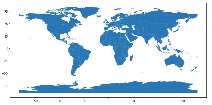
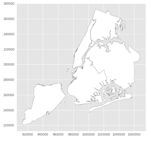
Geopandas uses matplotlib behind the scenes hence little background of matplotlib will be helpful with it as well. We'll start by just plotting the world dataframe which we loaded above to see results. We can simply call plot() on GeoDataFrame and it'll plot world countries on map. By default, it'll just print all countries with their borders. Below we are printing both world and new york maps.

We'll now load our world happiness data. Please feel free to download a dataset from kaggle.

Dataset URL: World Happiness Report

Dataset also holds information about GDP per capita, social support, life expectancy, generosity, and corruption. We'll be merging this dataframe with geopandas world GeoDataFrame which we loaded above to combine data and then use combined data for plotting. Please make a note that the happiness report dataset does not have a happiness report for all countries present on earth. It has data for around 156 countries.

NOTE: Please make a note that we have manually made changes to the happiness dataset for around 10-15 countries where the country name was mismatching with name present in geopandas geodataframe. We have modified happiness report CSV to have the same country name as that of the geodataframe.

NOTE: Please make a note that while combining normal dataframe to geodataframe we have used geodataframe first in merge operation. The main reason for doing so is that it'll output GeoDataFrame as output else it'll output normal pandas dataframe as output without geo functionalities. Please make a note that there will be few NANs present in the dataframe because we don't have happiness data for all countries of the world.

3. Choropleth Maps ¶

We'll now explain a few choropleth maps using the happiness dataset which we created above by combining geopandas world geodataframe with the world happiness report dataset.

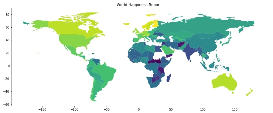
3.1 Happiness Choropleth Map ¶

Below we are plotting our first choropleth map by simply calling the plot() method on geopandas GeoDataFrame by passing a column name as the first parameter to use for the map. We can pass other arguments like figsize, edgecolor, edgesize, etc for map. As it is a static matplotlib plot, we can call other matplotlib methods like title(), xlabel(), ylabel(), etc will work on it.

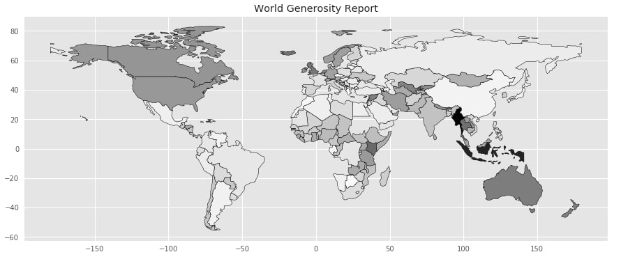
3.2 Generosity Choropleth Map ¶

Below we are generating another choropleth map using the Generosity column of the dataset. Please make a note that we are using the styling of seaborn and ggplot combined for this map as well.

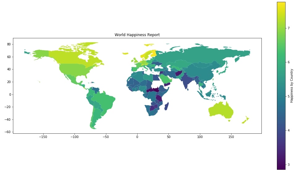
3.3 Happiness Choropleth Map with Legend ¶

We can also add legend and colormap to our choropleth map using the legend argument passed as True. We can also label our legend by passing arguments to the legend_kwds parameter.

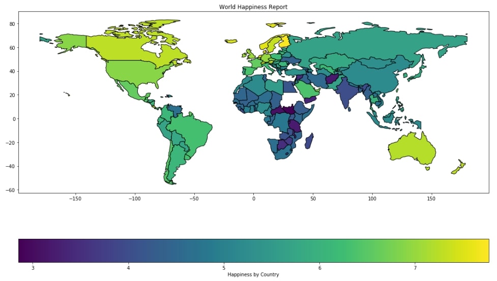
Below we are adding border as well to each country in choropleth map using edge color attribute. We are also moving colormap below by passing value orientation: horizontal to legend_kwds parameter.

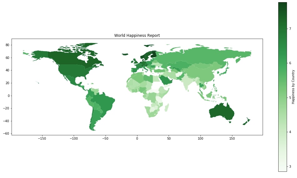
3.4 Happiness Choropleth Map with Legend & Different Colormaps ¶

We can change the default colormap of the choropleth map by passing different values for parameter cmap. It accepts a valid value from a list of available cmap values.

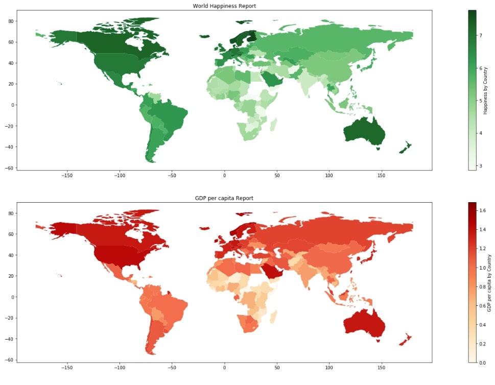
3.5 Multiple Choropleth Maps ¶

Below we are explaining another example where we can use a matplotlib axes system and can lay down more than one map plot in one image. We are plotting the choropleth map for Happiness and GDP Per Capita columns of data.

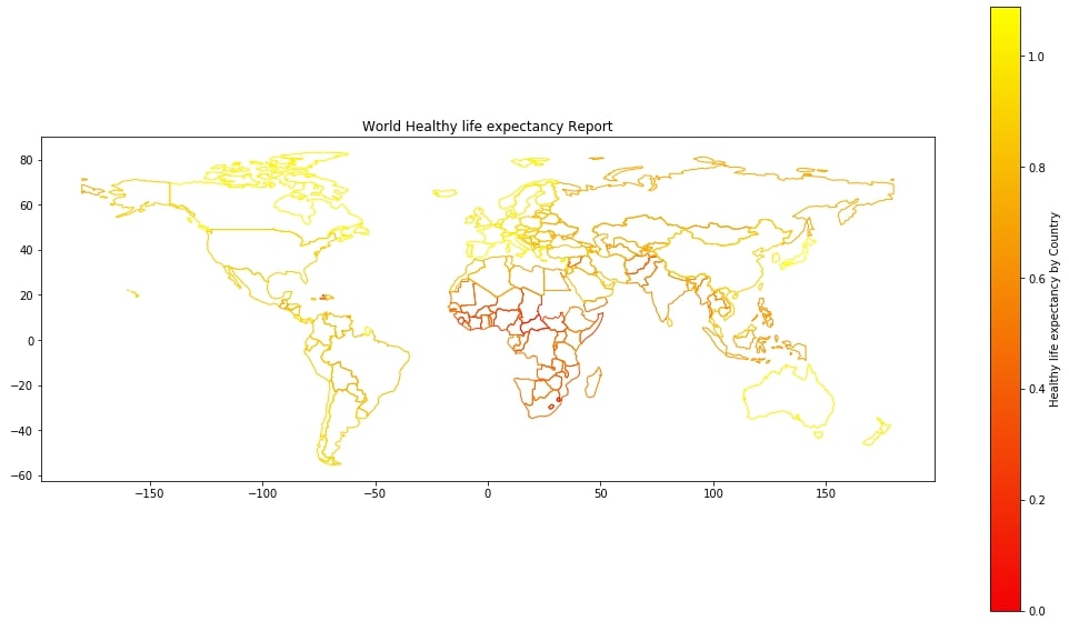
3.6 Happiness Choropleth Map with boundaries ¶

We can only highlight the boundaries of map plots without filling in any color. For this to work, we need to pass a special value none to parameter facecolor. Please make a note that we need to pass edgecolor as well which will be overridden with the color value of colormaps.

Below we are using healthy life expectancy as a column for plotting map.

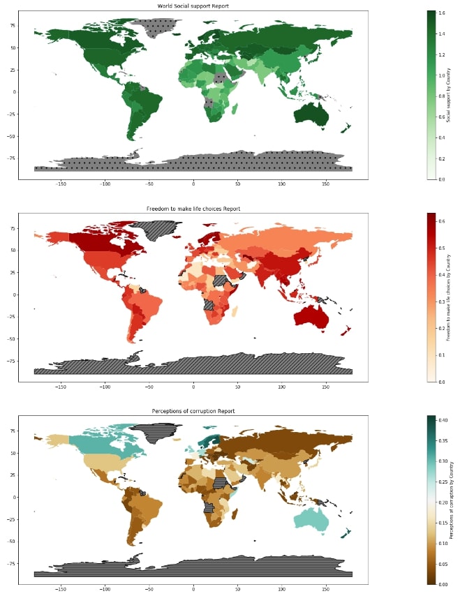
3.7 Choropleths Map with Missing Values handled ¶

It'll happen many times that we won't have data for all observations and we might want to highlight those observations for which we do not have values with different representations. We can use a parameter called missing_kwds passing it dictionary of a parameter on handling plotting of missing observation. Please make a note that this future is available from geopandas version 0.7 onwards only.

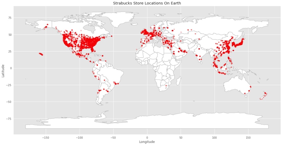
4. Scatter Plots on Maps ¶

We'll now explain scatter plots on maps with few examples. We'll use starbucks store location data available from kaggle for plotting these graphs. It has information about each Starbucks store locations as well as their address, city, country, phone number, latitude and longitude data.

Below we are plotting a simple map plot first and then using a scatter plot available in matplotlib to plot all Starbucks locations on it. Please make a note that we have longitude and latitude data for each store available in the dataset which we are utilizing in scatter plot.

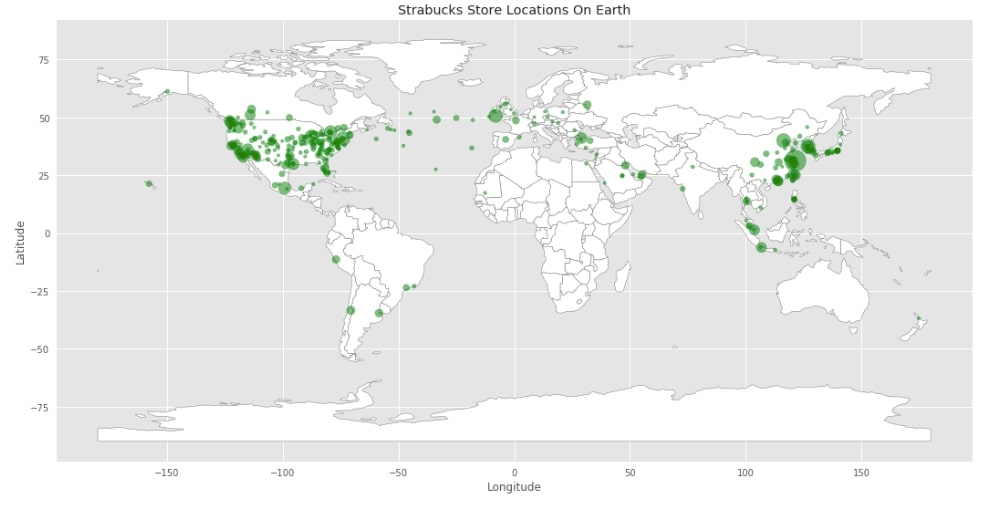
Below we are trying to get a count of Starbucks stores in each city of the world and then keeping only cities where more than 10 Starbucks are present per city. We are the first grouping data by the city to get average longitude and latitude. Then we generate another dataframe that has store count per city. We then combine dataframe with latitude & longitude with counts data. We only keep entries where more than 10 Starbucks is present.

Below we are plotting world map by default first and then overlapping scatter plot of cities where more than 10 Starbucks are present. We are using a number of Starbucks as size to represent Starbucks counts per city.

We'll be publishing another tutorial on working with geopandas where we'll be explaining how to use geopandas with other data file types like shape files and geojson files.

References ¶

• Maps using Folium
• Interactive Maps
• Maps using bqplot
• Maps using Cartopy
• Choropleth Maps and Scatter Maps using Cufflinks
• Plotting Maps using Bokeh
• ipyleaflet - Interactive Maps in Python based on leaflet.js
• Interactive Choropleth Maps using Bqplot
• Choropleth Maps using ipyleaflet
• Connection Maps using Plotly and Geopandas