Scikit-Learn: ML Model Evaluation Metrics (Classification, Regression, and Clustering Metrics)¶

Machine Learning and Artificial Intelligence are the most trending topics of 21st century. Everyone is trying different types of ML models to solve their tasks.

Many ML Models can help automate tasks that were otherwise needed manual actions. One just needs enough data to train ML model. There are many Python libraries (scikit-learn, statsmodels, xgboost, catbooost, lightgbm, etc) providing implementation of famous ML algorithms. With easy to use API of these libraries, it is very easy to train ML Models using them.

But how does one check whether their trained model is meeting expectations?

Whether model generalized or not?

Is it really good at task that we can automate things or find insights into?

How does one evaluate performance of ML Models for a given task?

That's where ML Metrics comes in.

> What is Machine Learning Model Evaluation Metric or ML Metric?¶

Machine Learning Metric or ML Metric is a measure of performance of an ML model on a given task. It helps us decide whether a model is good or we need to improve it. A task can be any ML task like classification, regression, clustering, etc.

ML Metric generally gives us a number that we can use to decide whether we should keep model or try another algorithm or perform hyperparameters tuning.

For classification tasks, it can be 'accuracy' that tells us how many labels were right. For regression tasks, it can mean absolute error, which tells us on average how far our predictions are from actual values.

There can be more than one metric that let us understand model performance better from different angles like accuracy, ROC AUC curve, confusion matrix, etc for classification tasks.

These metrics help us understand whether our ML model has generalized or not which can lead to better decision-making.

Python library scikit-learn (sklearn) which is first choice of many ML developers to try ML Models. It provides an implementation of many ML metrics.

> What Can You Learn From This Article?¶

As a part of this tutorial, we have explained how to use various ML Metrics available from scikit-learn through 'metrics' sub-module. It provides many metrics to measure performance of ML models. Tutorial covers various metrics available for classification, regression and clustering tasks. We have also explained how to create custom metrics.

In scikit-learn, the default choice for classification is 'accuracy' which is a number of labels correctly classified, and for regression is 'r2' which is a coefficient of determination.

Below, we have listed important sections of tutorial to give an overview of the material covered.

Important Sections Of Tutorial¶

1. Classification Metrics
   • 1.1 Load Data and Train Model
   • 1.2 Evaluate ML Metrics for Classification Tasks
     • 1 - Classification Accuracy
     • 2 - Confusion Matrix
     • 3 - Classification Report (Precision, Recall, and F1-Score)
     • 4 - ROC Curves
     • 5 - Precision-Recall Curve
     • 6 - Log Loss (Logistic Loss or Cross-Entropy Loss)
     • 7 - Zero One Classification Loss
     • 8 - Balanced Accuracy Score
     • 9 - Brier Loss
     • 10 - F-Beta Score
     • 11 - Hamming Loss
2. Regression Metrics
   • 2.1 Load Data and Train Model
   • 2.2 Evaluate ML Metrics for Regression Tasks
     • 1 - R2 Score (Coefficient Of Determination)
     • 2 - Mean Absolute Error
     • 3 - Mean Squared Error
     • 4 - Mean Squared Log Error
     • 5 - Median Absolute Error
     • 6 - Explained Variance Score
     • 7 - Residual Error
3. Clustering Metrics
   • 3.1 Load Data and Train Model
   • 3.2 Evaluate ML Metrics for Clustering Tasks
     • 1 - Adjusted Rand Score
4. How to Create Custom Metric/Scoring Function?
5. List of All Metrics available from Scikit-Learn

Below, we have imported necessary Python libraries for our tutorial and printed the versions of them used in tutorial.

1. Classification Metrics ¶

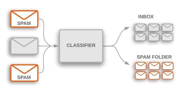
In this section, we'll explain various classification metrics available from scikit-learn. We'll train a simple classification model and then calculate various metrics to evaluate their performance.

If you want to learn about classification using scikit-learn then we recommend that you go through below link. It has detailed guidance on topic.

Supervised Learning: Classification using Scikit-Learn

1.1 Load Data and Train Model¶

We have loaded breast cancer dataset available from scikit-learn for this section. The dataset has various measurements of tumors as features and target variable is binary (malignant - 0, benign - 1). Dataset has 500+ examples, 30 features, and 2 target classes.

After loading dataset, we'll be splitting a dataset into train set(80% samples) and test set (20% samples).

We'll be using a simple LogisticRegression model for training purposes. We'll then proceed to introduce various classification metrics which will be evaluating model performance on test data from various angles.

1.2 Evaluate ML Metrics for Classification Tasks¶

1. Classification Accuracy¶

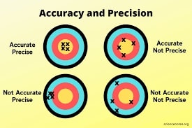
Accuracy is number of true predictions divided by total number of samples. It tells us percentage/portion of examples that were predicted correctly by model.

Scikit-learn has a function named 'accuracy_score()' that let us calculate accuracy of model. We need to provide actual labels and predicted labels to function and it'll return an accuracy score.

Also, all classification models by default calculate accuracy when we call their score() methods to evaluate model performance.

2. Confusion Matrix¶

For binary and multi-class classification problems, confusion matrix is another metric that helps in identifying which classes are easy to predict and which are hard to predict. It provides how many examples for each class are correctly classified and how many are confused with other classes.

Confusion Matrix for binary classification problems has the below-mentioned structure.

[[TN, FP ]
 [FN, TP ]]

• TN refers to True Negative which is the count of labels which were originally belonged to negative class and model also predicted them as negative.
• FP refers to False positive which is the count of labels which were actually belonged to negative class but model predicted them as positive.
• FN refers to False Negative which is the count of labels which were actually belonged to Positive Class but model predicted them as negative.
• TP refers to True Positive which is the count of labels predicted positive that were actually positive.

Scikit-learn provides us with function named 'confusion_matrix()' through 'metrics' module to calculate confusion matrix. We need to provide actual labels and predicted labels for it.

Below we are plotting the confusion matrix as it helps in interpreting results fast.

We have created a chart using Python library scikit-plot. It provides visualizations for many different ML Metrics. Please feel free to check below link to learn about it. We'll use it again below for some other ML metrics.

• Scikit-Plot: Visualize Evaluation Metrics of ML Models

3. Classification Report (Precision, Recall, and F1-Score)¶

Classification report metrics provide precision, recall, f1-score, and support for each class.

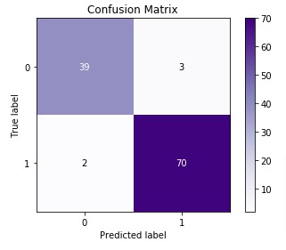
• Precision - It represents how many predictions of a particular class are actually of that class.
  • Precision = TP / (TP+FP).
• Recall - It represents how many predictions of a particular class are right.
  • Recall = TP / (TP+FN).
• f1-score - It's geometric average of precision & recall.
  • F1-Score = 2 (Precision recall) / (Precision + recall)
• support - It represents number of occurrences of particular class in Y_true

Below, we have included a visualization that gives an exact idea about precision and recall.

Scikit-learn provides various functions to calculate precision, recall and f1-score metrics.

1. precision_score() - Calculates overall precision.
2. recall_score() - Calculates overall recall.
3. f1-score() - Calculates overall f1-score.
4. precision_recall_fscore_support() - Calculates precision, recall and f1-score per target class.
5. classification_report() - Calculates precision, recall and f1-score per target class.

4. ROC Curves & ROC AUC¶

ROC(Receiver Operating Characteristic) Curve helps better understand the performance of the model when handling an unbalanced dataset.

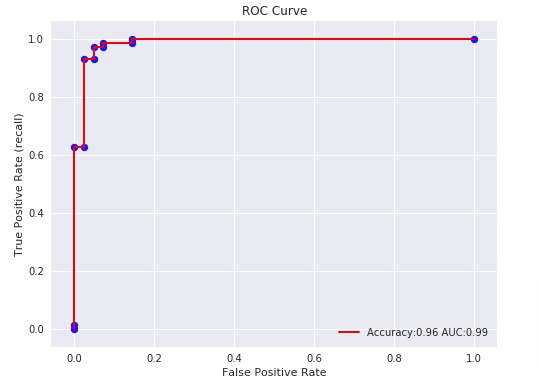
ROC Curve works with the output of prediction function or predicted probabilities by setting different threshold values to classify examples. It then calculates different false positives rates (FPR) and true positive rates (TPR) according to set threshold values. We can then plot a line chart with Y-axis as TPR and X-axis as FPR. The area under the line is generally referred to as ROC AUC (ROC Area Under Curve).

E.g., The output of binary classification model is probability in range 0-1. We can try different threshold values (0.2,0.35, 0.5, 0.65, 0.8, 0.95) to classify examples. Based on selected threshold value, the example with probability less than threshold is classified as negative class and greater than is classifier as positive class. This way we'll get different positives and negatives for each threshold.

In the case of SVC, for example, a threshold set for output of decision function is 0 whereas ROC Curve tries various values for thresholds like [2,1,-1,-2] including negative threshold values as well.

In the case of LogisticRegression, the default threshold is 0.5 and ROC will try different threshold values.

For linear regression, the output is a probability between [0,1] hence threshold is set at 0.5 to differentiate positive/negative classes whereas in case of SVC internal kernel function returns a value, and threshold is set on that value for making a prediction.

Note: It's restricted to binary classification tasks.

Scikit-learn provides various metrics to calculate ROC and ROC AUC metrics.

1. roc_curve() - It takes actual labels and output of decision_function() or predict_proba() as input. It then returns TPR and FPR along with different threshold values that were tried. We can create line plot explained earlier using these TPR and FPR values.
2. roc_auc_score() - It works like roc_curve() but returns area under the curve.

Below, we have explained how to calculate ROC & ROC AUC using sklearn. We can use either predict_proba() or decision_function() for calculation.

Below, we have plotted ROC using matplotlib.

Below, we have plotted ROC using Python library scikit-plot.

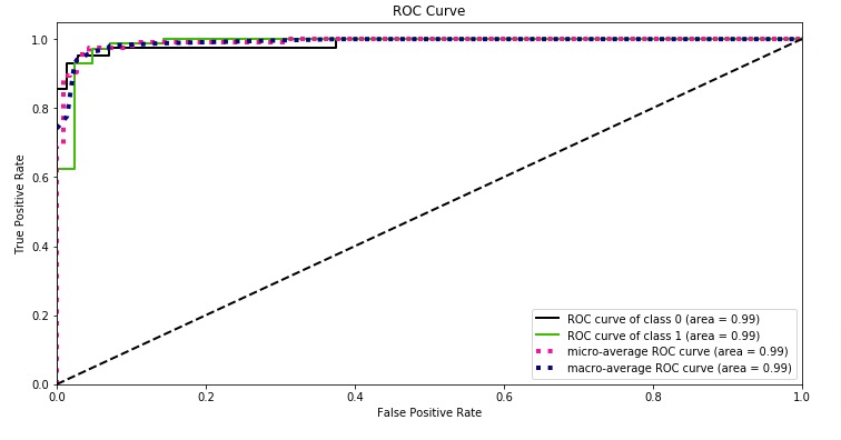
With a very small decision threshold, there will be few false positives, but also few false negatives, while with a very high threshold, both true positive rate and the false positive rate will be high.

So in general, the curve will be from the lower left to the upper right. A diagonal line reflects chance performance, while the goal is to be as much in the top left corner as possible. We want ROC Curve to cover almost 100% area for good performance. 50% area coverage refers to the chance model (random prediction).

5. Precision-Recall Curve¶

Precision and Recall help a lot in case of imbalanced datasets. It works exactly like ROC curve but uses precision and recall values.

Plotting different values of precision vs recall by setting different thresholds helps in evaluating the performance of the model better in case of imbalance classes. It does not take into consideration true negatives as it's majority class and True positives represent minority class which has quite a few occurrences.

Note: It's restricted to binary classification tasks.

Scikit-learn provides various metrics to calculate Precision-Recall Curve and Precision-Recall Curve AUC metrics.

1. precision_recall_curve() - It takes actual labels and output of decision_function() or predict_proba() as input. It then returns precision and recall along with different threshold values that were tried. We can create line plot explained earlier using these precision and recall values.
2. auc() - It works like precision_recall_curve() but returns area under the curve.

Below, we have explained how to calculate precision-recall curve & precision-recall AUC using sklearn. We can use either predict_proba() or decision_function() for calculation.

Below, we have plotted Precision Recall Curve using matplotlib.

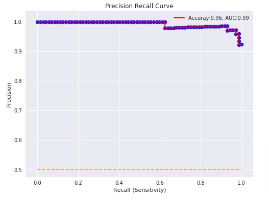
Below, we have plotted Precision Recall Curve using Python library scikit-plot.

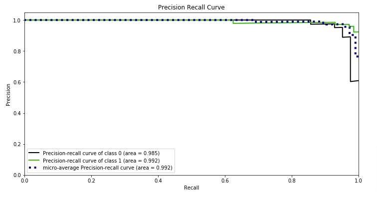
What to Use for Imbalanced Dataset (ROC AUC or Precision Recall AUC)?¶

Precision-recall curve totally crashes if our model is not performing well in case of an imbalanced dataset. ROC curves sometimes give optimistic results hence it's better to consider precision-recall curves as well in case of imbalanced datasets. We recommend looking at classification reports as well for imbalanced datasets.

6. Log Loss (Logistic Loss or Cross-Entropy Loss)¶

Log loss refers to the negative log-likelihood of true labels predicted by the classifier. It's a cost function whose output classifiers try to minimize while updating weights of the model.

log_loss = - y * log (y_probs) - (1-y) * log(1 - y_probs)

Scikit-learn provides a function named log_loss() through 'metrics' sub-module for calculating log loss. We need to provide actual target labels and predicted probabilities for calculating log loss to function.

7. Zero One Classification Loss¶

It returns a number of misclassifications or a fraction of misclassifications. It accepts normalize parameter whose value if set True then returns a fraction of misclassifications else if set to False then it returns misclassifications.

Scikit-learn provides function named 'zero_one_loss()' function through 'metrics' sub-module. We need to provide actual and predicted target labels to calculate zero one classification loss.

8. Balanced Accuracy Score¶

It returns an average recall of each class in classification problem. It's useful to deal with imbalanced datasets.

It has parameter adjusted which when set True results are adjusted for a chance so that the random performing model would get a score of 0 and perfect performance will get 1.0.

We can calculate balanced accuracy using 'balanced_accuracy_score()' function of 'sklearn.metrics' module. We need to provide actual and predicted labels to function.

9. Brier Loss¶

It computes squared differences between the actual labels of class and predicted probability by model. It should be as low as possible for good performance. It’s for binary classification problems only. It by default takes 1 as a positive class hence if one needs to consider 0 as a positive class then one can use the pos_label parameter as below.

We can calculate brier loss using 'brier_score_loss()' from scikit-learn. We need to provide actual target labels and predicted probabilities of positive class to it.

10. F-Beta Score¶

F-Beta score refers to a weighted average of precision and recall based on the value of the beta parameter provided. If beta < 1 then it lends more weight to precision, while beta > 1 lends more weight to recall. It has the best value of 1.0 and the worst 0.0.

It has a parameter called average which is required for multiclass problems. It accepts values [None, 'binary'(default), 'micro', 'macro', 'samples', 'weighted']. If None is specified then the score for each class is returned else average as per parameter is returned in a multi-class problem.

We can calculate F-beta score using fbeta_score() function of scikit-learn.

11. Hamming Loss¶

It returns a fraction of labels misclassified. We can calculate hamming loss using hamming_loss() function of scikit-learn.

2. Regression Metrics ¶

In this section, we'll introduce model evaluation metrics for regression tasks. We'll first train a simple regression model and then evaluate its performance by calculating various regression metrics.

If you want to learn how to handle regression tasks using scikit-learn then please check below link. It covers topic in detail.

Supervised Learning: Regression using Scikit-Learn

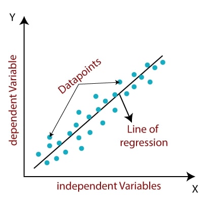
2.1 Load Data and Train Model¶

We'll start with loading the Boston dataset available in scikit-learn for our purpose.

We'll be splitting a dataset into train/test sets with 80% for a train set and 20% for the test set.

We'll now initialize a simple LinearSVR model and train it on the train dataset. We'll then check its performance by evaluating various regression metrics provided by scikit-learn.

2.2 Evaluate ML Metrics for Regression Tasks¶

1. R2 Score (Coefficient Of Determination)¶

The coefficient of R2 is defined as below.

The R2 score generally has values in the range 0-1. The values near 1 are considered signs of a good model.

The best possible score is 1.0 and it can be negative as well if the model is performing badly. A model that outputs constant prediction for each input will have a score of 0.0.

Scikit-learn provides function named 'r2_score()' through 'metrics' sub-module to calculate R2 score.

Below we are doing a grid search through various values of parameter C of LinearSVR and using r2 as an evaluation metric whose value will be optimized.

If you do not have a background on Grid search and want to learn about it then we would recommend you to check below link in your free time. It'll help you with the concept.

• Scikit-Learn: Hyperparameters Tuning Using Grid Search

2. Mean Absolute Error (MAE)¶

Mean absolute error is a simple sum of the absolute difference between actual and predicted target value divided by a number of samples.

Scikit-learn provides function named 'mean_absolute_error()' through 'metrics' sub-module to calculate mean absolute error.

Below we are doing a grid search through various values of parameter C of LinearSVR and using neg_mean_absolute_error as an evaluation metric whose value will be optimized.

3. Mean Squared Error (MSE)¶

Mean Squared Error loss function simple sum of the squared difference between actual and predicted values divided by a number of samples.

Scikit-learn provides function named 'mean_squared_error()' through 'metrics' sub-module to calculate mean squared error.

Below we are doing grid search through various values of parameter C of LinearSVR and using neg_mean_squared_error as an evaluation metric whose value will be optimized.

4. Mean Squared Log Error¶

It can not be used when target contains negative values/predictions.

Scikit-learn provides function named 'mean_squared_log_error()' through 'metrics' sub-module to calculate mean squared log error.

5. Median Absolute Error¶

Scikit-learn provides function named 'median_absolute_error()' through 'metrics' sub-module to calculate median absolute error.

6. Explained Variance Score¶

It returns the explained variance regression score. The best value is 1.0 and fewer values refer to a bad model.

Scikit-learn provides function named 'explained_variance_score()' through 'metrics' sub-module to calculate explained variance score.

7. Residual Error¶

It returns the max of the difference between actual values and the predicted value of all samples.

Scikit-learn provides function named 'max_error()' through 'metrics' sub-module to calculate residual error.

3. Clustering Metrics ¶

We'll now introduce evaluation metrics for unsupervised learning - clustering tasks. We'll train a simple ML model for solving clustering task and then evaluate its performance by calculating various metrics.

If you want to learn about clustering then we would recommend you to go through below link as it covers topic in detail.

Unsupervised Learning: Clustering using Scikit-Learn

3.1 Load Data and Train Model¶

3.2 Evaluate ML Metrics for Clustering Tasks¶

1. Adjusted Rand Score¶

Clustering algorithms return cluster labels for each cluster specified but they might not return in the same sequence as original labels. It might happen that in the original dataset some class has samples labeled as 1 and in predictions by cluster, an algorithm can label it as other than 1.

We'll use the IRIS dataset and KMeans for explanation purposes. We'll even plot results to show the difference. We'll show accuracy will improve once we use 'adjusted_rand_score()' as an evaluation function.

4. How to Create Custom Metric/Scoring Function? ¶

Users can also define their own scoring function if their scoring function is not available in built-in scoring functions of sklearn. In GridSearchCV and cross_val_score, one can provide object which has call method or function to scoring parameter. Object or function both need to accept estimator object, test features(X) and target(Y) as input, and return float.

Below we are defining RMSE (Root Mean Squared Error) as a class and as a function as well. We'll then use it in cross_val_score() to check performance also compares it's value with negative of neg_mean_squared_error.

Custom Metrics with Cross Validation¶

Below, we have explained how to use custom metrics with scikit-learn function cross_val_score().

If you are someone who does not have background on cross validation then we would recommend you to check below link.

• Scikit-Learn: Cross Validation

Custom Metrics with Grid Search¶

Below, we have explained how to use custom metrics with grid search.

If you are someone who does not have background on grid search then we would recommend you to check below link.

• Scikit-Learn: Hyperparameters Tuning Using Grid Search

5. List of All Metrics available from Scikit-Learn ¶

Below are list of scikit-learn builtin functions.

This ends our small tutorial explaining how to use various ML metrics available from 'metrics' sub-module of 'sklearn' to evaluate performance of ML Models trained on classification, regression and clustering tasks.

> Are ML Metrics Enough to Evaluate Model Performance?¶

Though ML Metrics are a good starting point for evaluating performance of ML Models, sometimes they are not enough. There can be situations when ML metrics are giving good numbers indicating a good model but in reality, our model has not generalized.

> Should you Interpret Predictions of Model?¶

That's where various algorithms to interpret predictions of ML models come in handy. They let us see which features are contributing to predictions. What is intensity of various features towards predictions? This can helps us make even more informed decisions.

We would recommend that you read our tutorials for interpreting predictions of ML Models listed below in references section as it'll help you evaluate model performance even better.

References¶

Libraries to Visualize ML Metrics¶

• Scikit-Plot: Visualize ML Metrics
• yellowbrick: Visualize Sklearn Classification and Regression Metrics
• yellowbrick: Text Data Visualizations

Python Libraries to Interpret Predictions of ML Models¶

• How to Use LIME to Interpret Predictions of ML Models?
• SHAP Values: Explain Predictions of ML Models using Game-Theoretic Approach
• How to Use 'Eli5' to Understand ML Models and their Predictions?
• captum: Interpret Predictions of PyTorch Networks
• Treeinterpreter: Interpreting Tree-Based Model's Prediction of Individual Sample
• interpret-ml: Explain ML Models and their Predictions
• interpret-text: Explain NLP Models
• dice-ml: Diverse Counterfactual Explanations for ML Models