Scikit-Learn - Incremental Learning for Large Datasets
Scikit-Learn is one of the most widely used machine learning libraries of Python. It has an implementation for the majority of ML algorithms which can solve tasks like regression, classification, clustering, dimensionality reduction, scaling, and many more related to ML.
> Why Scikit-Learn is so Famous?
Scikit-learn has been accepted by the wide community due to its simple and easy-to-use API. It does not require developers to have a deep understanding of how a particular ML algorithm works. The developer can simply train their data with an ML algorithm with very few lines of code. It also lets us set up the whole machine learning pipeline and perform grid search for hyperparameters tunning with very ease.
> Majority of Scikit-Learn ML Models Supports Dataset that Fits into Main Memory of Computer
The main drawback with the majority of ML algorithms available through scikit-learn is that they require total data required for training in the main memory. The datasets available nowadays for the majority of the tasks have a lot of data and generally do not fit into the main memory of the computer.
The deep neural network learning libraries like Pytorch, tensorflow, keras, chainer, etc let us perform a training process on a batch of data and requires only a single batch of data into main memory at the time. This approach does not require all the data to be in the main memory instead only a small portion of it.
> How to Train "Scikit-Learn" ML Models with Dataset that Does not Fit into Main Memory? | How to Handle Datasets that Do not Fit into Main Memory of Computer using Scikit-learn?
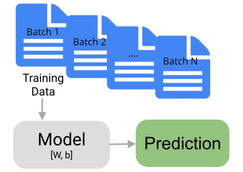
To solve this problem, scikit-learn provides a bunch of estimators which let us perform partial fit on data by using only a small batch of data. The model will be trained incrementally where we loop through the whole dataset in batches. It'll update model weights for each batch of data.
We can use these estimators in situations where our training data is so large that it does not fit into the main memory of the computer. We can create batches of data and bring the batch which fits into the main memory of our computer.
The scikit-learn estimators which support this feature provide one extra method named 'partial_fit()' which lets us perform the partial fit. The fit() method works on whole data and update model weights only once whereas "partial_fit()" updates for each batch.
Please make a NOTE that not all estimators/models available from scikit-learn has partial_fit() method. We have listed estimators below in the first section that supports it.
> What Can You Learn From This Article?
As a part of this tutorial, we'll be explaining how to train "scikit-learn" ML Models/estimators on datasets that do not fit into main memory of computer using partial_fit() method. We'll be explaining one estimator for each type of ML task (regression, classification, clustering, and dimensionality reduction) with simple examples. We'll be using toy datasets for our purposes to keep examples easy to grasp.
Below we have listed important sections of the tutorial to give an overview of the content that we'll be covering.
Important Sections of Tutorial
- List of Estimators with "partial_fit()" Method
- Regression
- Load Dataset
- Create and Train Model
- Evaluate Model Performance on Test Data (Calculate ML Metrics)
- Evaluate Model Performance on Train Data (Calculate ML Metrics)
- Classification
- Clustering
- Preprocessing
- Decomposition / Dimensionality Reduction
import sklearn

print("Scikit-Learn Version : {}".format(sklearn.__version__))
1. List of Estimators with "partial_fit()" Method 
Below we have listed estimators which have partial_fit() method available with them.
- Regression
- sklearn.linear_model.SGDRegressor
- sklearn.linear_model.PassiveAggressiveRegressor
- sklearn.neural_network.MLPRegressor
- Classification
- sklearn.naive_bayes.MultinomialNB
- sklearn.naive_bayes.BernoulliNB
- sklearn.linear_model.Perceptron
- sklearn.linear_model.SGDClassifier
- sklearn.linear_model.PassiveAggressiveClassifier
- sklearn.neural_network.MLPClassifier
- Clustering
- sklearn.cluster.MiniBatchKMeans
- sklearn.cluster.Birch
- Preprocessing
- sklearn.preprocessing.StandardScaler
- sklearn.preprocessing.MinMaxScaler
- sklearn.preprocessing.MaxAbsScaler
- Decomposition / Dimensionality Reduction
- sklearn.decomposition.MiniBatchDictionaryLearning
- sklearn.decomposition.IncrementalPCA
- sklearn.decomposition.LatentDirichletAllocation
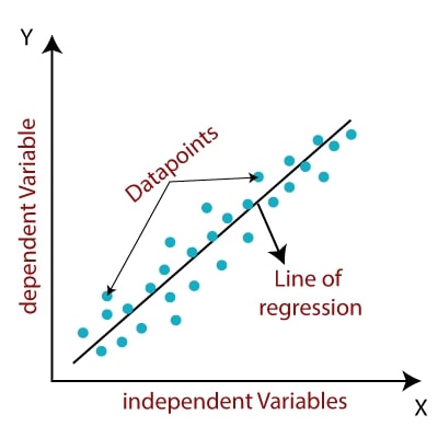
2. Regression 
In this section, we'll explain how we can perform incremental learning when we have large data. We'll be creating an artificial dataset for the regression task which will be large enough so that we'll be giving a small batch of that data to model for each training loop. We'll also evaluate model performance after training.
Below is a list of available regression estimators from scikit-learn which supports partial fit on a batch of data for datasets that do not fit into the main memory of the computer.
- sklearn.linear_model.SGDRegressor
- sklearn.linear_model.PassiveAggressiveRegressor
- sklearn.neural_network.MLPRegressor
If you are interested in learning about regression available from scikit-learn on small datasets which fit in the main memory of the computer then please feel free to check our tutorial on the same.
2.1 Load Dataset
In this section, we have created a regression dataset with 240,000 samples and 100 features using make_regression() method of scikit-learn. We have then divided dataset into train (90%) and test (10%) sets using train_test_split() method.
After dividing the dataset, we have reshaped the dataset in a way that new reshaped data will have 24 examples per batch. Each batch will have 24 examples. We'll be looping through this new reshaped data which will have 24 examples for each entry. We'll pretend that we are not able to fit this data into the main memory and bring only 24 examples of data at a time into the main memory.
from sklearn import datasets
from sklearn.model_selection import train_test_split

X, Y = datasets.make_regression(n_samples=240000, random_state=123)

X_train, X_test, Y_train, Y_test = train_test_split(X, Y, train_size=0.9, random_state=123)

X_train.shape, X_test.shape, Y_train.shape, Y_test.shape
X_train, X_test = X_train.reshape(-1,24,100), X_test.reshape(-1,24,100)
Y_train, Y_test = Y_train.reshape(-1,24), Y_test.reshape(-1,24)

X_train.shape, X_test.shape, Y_train.shape, Y_test.shape
X_train[0].shape, Y_train[0].shape
2.2 Create and Train Model
In this section, we have created an ML model using SGDRegressor class of scikit-learn. We have then looped through data in batches and trained this estimator by calling partial_fit() method on it for each batch of data. We have also looped through total data 10 times where each time training will be performed in batches.
Below we have included a definition of SGDRegressor estimator for explanation purposes.
- SGDRegressor(loss='squared_error',penalty='l2', alpha=0.0001, l1_ratio=0.15, fit_intercept=True, max_iter=1000, tol=0.001, shuffle=True, verbose=0, epsilon=0.1, random_state=None, learning_rate='invscaling', eta0=0.01, power_t=0.25, early_stopping=False, validation_fraction=0.1,warm_start=False) - This class creates linear model for regression task.
- The loss parameter accepts one of the below strings specifying loss.
- 'squared_error'
- 'huber'
- 'epsilon_insensitive'
- 'squared_epsilon_insensitive'
- The penalty parameter accepts string specifying penalty. The possible values of the parameters are 'l2', 'l1' and 'elasticnet'. The default is 'l2'.
- The l1_ratio parameter accepts float value in the range [0,1] specifying the amount of l1 penalty to use for elasticnet penalty which is a mix of l1 and l2. If a float value of 0 is specified then only l2 penalty is used and a value of 1.0 specifies only the l1 penalty. The value between 0 and 1 specifies the combination of l1 and l2.
- The fit_intercept parameter accepts boolean values specifying whether to include an intercept in the model or not.
- The learning_rate parameter accepts one of the below-mentioned strings specifying the learning rate.
- 'constant'
- 'optimal'
- 'invscaling'
- 'adaptive'
- The validation_fraction parameter accepts float in the range 0-1 specifying how much of training sample should be used for validation. The default is 0.1 which means that 10% of training samples will be used for validation purposes.
- The loss parameter accepts one of the below strings specifying loss.
Below we have created an instance of SGDRegressor with the default parameter. We have then looped through data in batches and called partial_fit() on regressor instance with each batch. We have performed this process for 10 epochs which means we have looped through total training data 10 times in batches.
from sklearn.linear_model import SGDRegressor

regressor = SGDRegressor()

epochs = 10

for k in range(epochs): ## Number of loops through data
    for i in range(X_train.shape[0]): ## Looping through batches
        X_batch, Y_batch = X_train[i], Y_train[i]
        regressor.partial_fit(X_batch, Y_batch) ## Partially fitting data in batches
2.3 Evaluate Model Performance on Test Data
In this section, we have evaluated the performance of our trained model on test data. We have looped through test data in batches and made predictions on them. We have then combined the prediction of each batch.
At last, we have calculated MSE and R^2 scores on the test dataset to check the performance of the model.
If you are interested in learning about model evaluation metrics using scikit-learn then please feel free to check our tutorial on the same which explains the topic with simple and easy-to-understand examples.
from sklearn.metrics import mean_squared_error, r2_score


Y_test_preds = []
for j in range(X_test.shape[0]): ## Looping through test batches for making predictions
    Y_preds = regressor.predict(X_test[j])
    Y_test_preds.extend(Y_preds.tolist())

print("Test MSE      : {}".format(mean_squared_error(Y_test.reshape(-1), Y_test_preds)))
print("Test R2 Score : {}".format(r2_score(Y_test.reshape(-1), Y_test_preds)))
2.4 Evaluate Model Performance on Train Data
In this section, we have evaluated the performance of our trained model on train data. We have looped through train data in batches and made predictions. We have combined predictions of each batch.
At last, we have calculated MSE and R^2 scores on the training dataset to check the performance of the model on train data.
from sklearn.metrics import mean_squared_error, r2_score

Y_train_preds = []
for j in range(X_train.shape[0]): ## Looping through train batches for making predictions
    Y_preds = regressor.predict(X_train[j])
    Y_train_preds.extend(Y_preds.tolist())

print("Train MSE      : {}".format(mean_squared_error(Y_train.reshape(-1), Y_train_preds)))
print("Train R2 Score : {}".format(r2_score(Y_train.reshape(-1), Y_train_preds)))
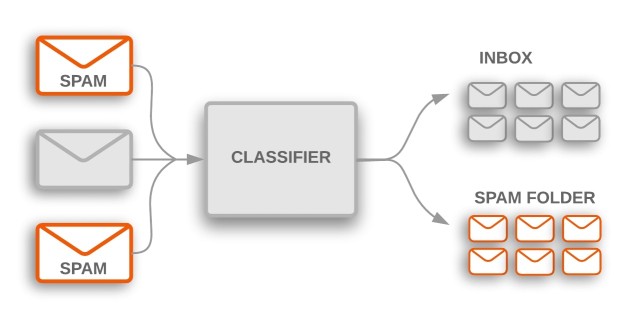
3. Classification 
In this section, we'll explain how we can perform incremental learning with large data for classification tasks. We'll be creating an artificial dataset using scikit-learn methods and then training a classification model on it.
Below is a list of available classification estimators from scikit-learn which supports partial fit on a batch of data for datasets that do not fit into the main memory of the computer.
- sklearn.naive_bayes.MultinomialNB
- sklearn.naive_bayes.BernoulliNB
- sklearn.linear_model.Perceptron
- sklearn.linear_model.SGDClassifier
- sklearn.linear_model.PassiveAggressiveClassifier
- sklearn.neural_network.MLPClassifier
If you are interested in learning about classification models available from scikit-learn for datasets that fit into the main memory of the computer then please feel free to check our tutorial on the same which explains it with simple examples.
3.1 Load Data
In this section, we have first created a classification dataset with 32k samples and 30 features using make_classification() method of scikit-learn. Our dataset has two classes which we'll be predicting using our classification model.
After dataset creation, we have divided the dataset into the train (90%) and test (10%) sets.
We have then reshaped train and test datasets so that there are batches of 32 examples in each entry of the dataset. We'll be looping through our dataset into batches of size 32 examples during training. This will help us imitate the behavior that we are able to fit only 32 examples of data into the main memory of the computer.
from sklearn import datasets
from sklearn.model_selection import train_test_split

X, Y = datasets.make_classification(n_samples=32000, n_features=30, n_informative=20, n_classes=2)

X_train, X_test, Y_train, Y_test = train_test_split(X, Y, train_size=0.9, random_state=123)

X_train.shape, X_test.shape, Y_train.shape, Y_test.shape
X_train, X_test = X_train.reshape(-1,32,30), X_test.reshape(-1,32,30)
Y_train, Y_test = Y_train.reshape(-1,32), Y_test.reshape(-1,32)

X_train.shape, X_test.shape, Y_train.shape, Y_test.shape
3.2 Create and Train Model
In this section, we'll create an SGDClassifier estimator and train it with data in batches. Below we have included a definition of it which is almost the same as SGDRegressor with a few minor changes.
- SGDClassifier(loss='hinge',penalty='l2', alpha=0.0001, l1_ratio=0.15, fit_intercept=True, max_iter=1000, tol=0.001, shuffle=True, verbose=0, epsilon=0.1, random_state=None, learning_rate='optimal', eta0=0.0, power_t=0.5, early_stopping=False, validation_fraction=0.1,warm_start=False) - This will create linear classifier which we can use for classification task.
- The loss parameter accepts one of the below strings specifying loss.
- 'hinge'
- 'log'
- 'modified_huber'
- 'squared_hinge'
- 'perceptron'
- The penalty parameter accepts string specifying penalty. The possible values of the parameters are 'l2', 'l1' and 'elasticnet'. The default is 'l2'.
- The l1_ratio parameter accepts float value in the range [0,1] specifying the amount of l1 penalty to use for elasticnet penalty which is a mix of l1 and l2. If a float value of 0 is specified then only l2 penalty is used and a value of 1.0 specifies only the l1 penalty. The value between 0 and 1 specifies the combination of l1 and l2.
- The fit_intercept parameter accepts boolean values specifying whether to include an intercept in the model or not.
- The learning_rate parameter accepts one of the below-mentioned strings specifying the learning rate.
- 'constant'
- 'optimal'
- 'invscaling'
- 'adaptive'
- The validation_fraction parameter accepts float in the range 0-1 specifying how much of training sample should be used for validation. The default is 0.1 which means that 10% of training samples will be used for validation purposes.
- The loss parameter accepts one of the below strings specifying loss.
Our code first creates an instance of SGDClassifier with default parameters. We then loop through training data in batches and partial fit classifier on the batch of data using partial_fit() method. We are looping through data for 10 epochs which means that we are looping through whole training data 10 times in batches.
from sklearn.linear_model import SGDClassifier

classifier = SGDClassifier(random_state=123)

epochs = 10

for k in range(epochs):
    for i in range(X_train.shape[0]):
        X_batch, Y_batch = X_train[i], Y_train[i]
        classifier.partial_fit(X_batch, Y_batch, classes=list(range(2))) ## Partially fitting data in batches
3.3 Evaluate Model on Test Data
In this section, we have evaluated the performance of test data by calculating the accuracy of the model. We are looping through test data in batches making predictions for each batch. We have then combined all batches’ predictions. At last, we have calculated the accuracy of test data and printed it.
from sklearn.metrics import accuracy_score


Y_test_preds = []
for j in range(X_test.shape[0]): ## Looping through test batches for making predictions
    Y_preds = classifier.predict(X_test[j])
    Y_test_preds.extend(Y_preds.tolist())

print("Test Accuracy      : {}".format(accuracy_score(Y_test.reshape(-1), Y_test_preds)))
3.4 Evaluate Model on Train Data
In this section, we have evaluated model performance on train data by calculating accuracy on it. We have looped through train data in batches making predictions for each batch. We have then calculated accuracy and printed it.
from sklearn.metrics import accuracy_score


Y_train_preds = []
for j in range(X_train.shape[0]): ## Looping through train batches for making predictions
    Y_preds = classifier.predict(X_train[j])
    Y_train_preds.extend(Y_preds.tolist())

print("Train Accuracy      : {}".format(accuracy_score(Y_train.reshape(-1), Y_train_preds)))
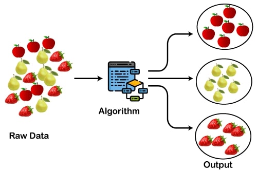
4. Clustering 
In this section, we'll explain how we can perform clustering on a dataset that is too large and does not fit into the main memory of the computer. We'll be creating a large dataset to mimic a real-life dataset and use one of the incremental estimators available from scikit-learn for clustering this large dataset.
Below is a list of available clustering estimators from scikit-learn which supports partial fit on a batch of data for datasets that do not fit into the main memory of the computer.
- sklearn.cluster.MiniBatchKMeans
- sklearn.cluster.Birch
If you are interested in learning about clustering models available from scikit-learn for datasets that fit into the main memory of the computer then please feel free to check our tutorials on the same which cover a topic with simple examples.
4.1 Load Data
In this section, we have created a classification dataset with 30 features and 5 clusters using make_blos() method of scikit-learn. We have created a dataset with 32k entries. After creating a dataset, we have split it into the train (90%) and test (10%) sets. We have then reshaped the train and test dataset in a way that each entry has 32 data examples. These 32 data examples will be considered one batch of data on which we'll train our model. We'll pretend that our dataset is quite big and we can only fit 32 examples into the main memory of the computer.
from sklearn import datasets
from sklearn.model_selection import train_test_split

X, Y = datasets.make_blobs(n_samples=32000, n_features=30, centers=5, cluster_std=0.7, random_state=12345)

X_train, X_test, Y_train, Y_test = train_test_split(X, Y, train_size=0.9, random_state=123)

X_train.shape, X_test.shape, Y_train.shape, Y_test.shape
X_train, X_test = X_train.reshape(-1,32,30), X_test.reshape(-1,32,30)
Y_train, Y_test = Y_train.reshape(-1,32), Y_test.reshape(-1,32)

X_train.shape, X_test.shape, Y_train.shape, Y_test.shape
4.2 Create and Train Model
In this section, we have created a scikit-learn estimator named MiniBatchKMeans() which lets us perform incremental clustering. We have given a number of clusters at the beginning when creating an estimator.
After creating the estimator, we are looping through the dataset, taking one batch of data, and training the estimator by calling partial_fit() method. We are looping through data for 10 epochs which means that we are making 10 pass-through data in batches of 32 samples.
from sklearn.cluster import MiniBatchKMeans

clustering_algo = MiniBatchKMeans(n_clusters=5, random_state=123)

epochs = 10

for k in range(epochs):
    for i in range(X_train.shape[0]):
        X_batch, Y_batch = X_train[i], Y_train[i]
        clustering_algo.partial_fit(X_batch, Y_batch) ## Partially fitting data in batches
4.3 Evaluate Model on Test Data
In this section, we are evaluating the performance of the estimator on the test dataset by using metrics available from scikit-learn. We are looping through test data in batches and making predictions for each batch at a time. We have then combined results from all batches.
We have then calculated the performance of the estimator by using adjusted_rand_score() metric available from scikit-learn. This estimator calculates the accuracy of the clustering estimator by adjusting the class labels predicted.
from sklearn.metrics import adjusted_rand_score


Y_test_preds = []
for j in range(X_test.shape[0]): ## Looping through test batches for making predictions
    Y_preds = clustering_algo.predict(X_test[j])
    Y_test_preds.extend(Y_preds.tolist())

print("Test Accuracy      : {}".format(adjusted_rand_score(Y_test.reshape(-1), Y_test_preds)))
4.4 Evaluate Model on Train Data
In this section, we have evaluated the performance of the clustering estimator on the training dataset. We have followed the same process which we followed for test accuracy calculation in the previous section.
from sklearn.metrics import adjusted_mutual_info_score


Y_train_preds = []
for j in range(X_train.shape[0]): ## Looping through train batches for making predictions
    Y_preds = clustering_algo.predict(X_train[j])
    Y_train_preds.extend(Y_preds.tolist())

print("Train Accuracy      : {}".format(adjusted_rand_score(Y_train.reshape(-1), Y_train_preds)))
5. Preprocessing 
In this section, we'll explain how we can perform preprocessing (scaling) on datasets that do not fit into the main memory of the computer. We'll be creating a big dataset and then training the scaling estimator on it in batches. After training the scaling estimator, we'll scale the dataset and also fit an estimator on the dataset to evaluate the performance. We'll be creating a regression dataset and train estimator which we used in the regression section.

Below is a list of available preprocessing estimators from scikit-learn which supports partial fit on a batch of data for datasets that do not fit into the main memory of the computer.
- sklearn.preprocessing.StandardScaler
- sklearn.preprocessing.MinMaxScaler
- sklearn.preprocessing.MaxAbsScaler
If you want to learn about preprocessing estimators available from scikit-learn for datasets that fit into the main memory of the computer then please feel free to check our tutorial on it which covers a topic with simple examples.
5.1 Load Data
In this section, we have created a regression dataset with 240k samples. The dataset has 100 features. We have then divided the dataset into the train (90%) and test (10%) sets. Then in the next cell, we have reshaped the dataset so that each entry of data has 24 examples. The code in this part is exactly the same as that of from regression section.
from sklearn import datasets
from sklearn.model_selection import train_test_split

X, Y = datasets.make_regression(n_samples=240000, random_state=123)

X_train, X_test, Y_train, Y_test = train_test_split(X, Y, train_size=0.9, random_state=123)

X_train.shape, X_test.shape, Y_train.shape, Y_test.shape
X_train, X_test = X_train.reshape(-1,24,100), X_test.reshape(-1,24,100)
Y_train, Y_test = Y_train.reshape(-1,24), Y_test.reshape(-1,24)

X_train.shape, X_test.shape, Y_train.shape, Y_test.shape
5.2 Create and Train Model After Scaling Data
In this section, we have first created an instance of StandardScaler which supports partial scaling of data. After creating a scaling estimator, we are looping through train data in batches and trained scaling estimator by calling partial_fit() on it with a single batch of data.
After the scaling estimator is trained, we have created an instance of SGDRegressor which we'll use for training scaled data. We are then looping through the dataset in batches taking a single batch at a time, scaling it with a scaling estimator, and training the regressor on scaled batch data using partial_fit() method.
from sklearn.linear_model import SGDRegressor
from sklearn.preprocessing import StandardScaler

### Scaling Data

scaler = StandardScaler()

for i in range(X_train.shape[0]):
    X_batch, Y_batch = X_train[i], Y_train[i]
    scaler.partial_fit(X_batch, Y_batch) ## Partially fitting data in batches


### Fitting Data in batches
regressor = SGDRegressor()

epochs = 10

for k in range(epochs):
    for i in range(X_train.shape[0]):
        X_batch, Y_batch = X_train[i], Y_train[i]
        X_batch = scaler.transform(X_batch) ## Preprocessing Single batch of data
        regressor.partial_fit(X_batch, Y_batch) ## Partially fitting data in batches
5.3 Evaluate Model Performance on Test Data
In this section, we are evaluating the performance of the regression estimator on the test dataset after scaling it. We are looping through data in batches taking a single batch of test data at a time, scaling the batch data, and then making predictions on scaled batch data. We have then combined the results of each batch of test data. We have calculated MSE and R^2 scores on the test dataset.
from sklearn.metrics import mean_squared_error, r2_score


Y_test_preds = []
for j in range(X_test.shape[0]): ## Looping through test batches for making predictions
    X_batch = scaler.transform(X_test[j]) ## Preprocessing Single batch of data
    Y_preds = regressor.predict(X_batch)
    Y_test_preds.extend(Y_preds.tolist())

print("Test MSE      : {}".format(mean_squared_error(Y_test.reshape(-1), Y_test_preds)))
print("Test R2 Score : {}".format(r2_score(Y_test.reshape(-1), Y_test_preds)))
5.4 Evaluate Model Performance on Train Data
In this section, we have evaluated the performance of regression on train data after scaling it. We have followed the same process which we did for the test dataset above.
from sklearn.metrics import mean_squared_error, r2_score

Y_train_preds = []
for j in range(X_train.shape[0]): ## Looping through train batches for making predictions
    X_batch = scaler.transform(X_train[j]) ## Preprocessing Single batch of data
    Y_preds = regressor.predict(X_batch)
    Y_train_preds.extend(Y_preds.tolist())

print("Train MSE      : {}".format(mean_squared_error(Y_train.reshape(-1), Y_train_preds)))
print("Train R2 Score : {}".format(r2_score(Y_train.reshape(-1), Y_train_preds)))
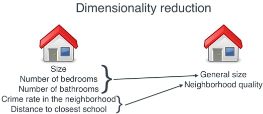
6. Decomposition / Dimensionality Reduction 
In this section, we'll explain how we can perform dimensionality reduction on datasets that do not fit into the main memory of the computer. We'll create a big dataset and train a dimensionality reduction estimator on it by giving a single batch of data. The single batch of data will have a few samples from our data which fits into the main memory of the computer. We'll then perform dimensionality reduction on this data and train an estimator on the dimensionality-reduced dataset. We'll then evaluate the performance of the estimator on dimensionality-reduced data.
Below is a list of available decomposition estimators from scikit-learn which supports partial fit on a batch of data for datasets that do not fit into the main memory of the computer.
- sklearn.decomposition.MiniBatchDictionaryLearning
- sklearn.decomposition.IncrementalPCA
- sklearn.decomposition.LatentDirichletAllocation
If you want to learn about decomposition/ dimensionality reduction estimators available from scikit-learn for datasets that fit into the main memory of the computer then please feel free to check our tutorial on it which covers a topic with simple examples.
6.1 Load Data
In this section, we have created a classification dataset with 30 features and 2 classes using make_classification() method of scikit-learn. Our dataset has 32k samples. We'll then divide the dataset into the train (90%) and test (10%) sets. After that, we'll reshape data so that a single entry of the dataset has 32 examples of data. We'll pretend that we are only able to fit these 32 examples at a time in the main memory. The code in this part is almost the same as that from the classification section.
from sklearn import datasets
from sklearn.model_selection import train_test_split

X, Y = datasets.make_classification(n_samples=32000, n_features=30, n_informative=20, n_classes=2, random_state=123)

X_train, X_test, Y_train, Y_test = train_test_split(X, Y, train_size=0.9, random_state=123)

X_train.shape, X_test.shape, Y_train.shape, Y_test.shape
X_train, X_test = X_train.reshape(-1,32,30), X_test.reshape(-1,32,30)
Y_train, Y_test = Y_train.reshape(-1,32), Y_test.reshape(-1,32)

X_train.shape, X_test.shape, Y_train.shape, Y_test.shape
6.2 Create and Train Model After Dimensionality Reduction
In this section, we have first created an instance of IncrementalPCA dimensionality reduction estimator with 20 components. This estimator will reduce our 30 features dataset to 20 features. We are then looping through train data in batches and training this dimensionality reduction estimator.
After completion of the training dimensionality reduction estimator, we have created an instance of SGDClassifier classification estimator. We have then again looped through train data in batches, reduced dimension of a single batch of data, and then trained regression estimator on this reduced dimension batch of data.
from sklearn.linear_model import SGDClassifier
from sklearn.decomposition import IncrementalPCA

### Scaling Data

pca = IncrementalPCA(n_components=20)

for i in range(X_train.shape[0]):
    X_batch, Y_batch = X_train[i], Y_train[i]
    pca.partial_fit(X_batch, Y_batch) ## Partially fitting data in batches


### Fitting Data in batches
classifier = SGDClassifier()

epochs = 20

for k in range(epochs):
    for i in range(X_train.shape[0]):
        X_batch, Y_batch = X_train[i], Y_train[i]
        X_batch = pca.transform(X_batch) ## Preprocessing Single batch of data
        classifier.partial_fit(X_batch, Y_batch, classes=list(range(2))) ## Partially fitting data in batches
6.3 Evaluate Model Performance on Test Data
In this section, we have evaluated the performance of the regressor on the reduced dimension test dataset. We are looping through train data in batches, reducing the dimension of each batch, and making predictions on a batch of reduced dimension data. We are then calculating the accuracy of the test dataset once all test sample prediction is done.
from sklearn.metrics import accuracy_score


Y_test_preds = []
for j in range(X_test.shape[0]): ## Looping through test batches for making predictions
    X_batch = pca.transform(X_test[j]) ## Preprocessing Single batch of data
    Y_preds = classifier.predict(X_batch)
    Y_test_preds.extend(Y_preds.tolist())

print("Test Accuracy      : {}".format(accuracy_score(Y_test.reshape(-1), Y_test_preds)))
6.4 Evaluate Model Performance on Train Data
In this section, we are evaluating the performance of the regressor on the reduced dimension train dataset. The process is exactly the same as our code from the previous cell with the only difference being that we are doing it on the training dataset in batches this time.
from sklearn.metrics import accuracy_score


Y_train_preds = []
for j in range(X_train.shape[0]): ## Looping through train batches for making predictions
    X_batch = pca.transform(X_train[j]) ## Preprocessing Single batch of data
    Y_preds = classifier.predict(X_batch)
    Y_train_preds.extend(Y_preds.tolist())

print("Train Accuracy      : {}".format(accuracy_score(Y_train.reshape(-1), Y_train_preds)))
This ends our small tutorial explaining how we can perform incremental learning on datasets that do not fit into the main memory of a computer and which estimators are available from scikit-learn for this kind of partial learning.
References
 Sunny Solanki
Sunny Solanki
Intro: Software Developer | Youtuber | Bonsai Enthusiast
About: Sunny Solanki holds a bachelor's degree in Information Technology (2006-2010) from L.D. College of Engineering. Post completion of his graduation, he has 8.5+ years of experience (2011-2019) in the IT Industry (TCS). His IT experience involves working on Python & Java Projects with US/Canada banking clients. Since 2020, he’s primarily concentrating on growing CoderzColumn.
His main areas of interest are AI, Machine Learning, Data Visualization, and Concurrent Programming. He has good hands-on with Python and its ecosystem libraries.
Apart from his tech life, he prefers reading biographies and autobiographies. And yes, he spends his leisure time taking care of his plants and a few pre-Bonsai trees.
Contact: sunny.2309@yahoo.in


![YouTube Subscribe]() Comfortable Learning through Video Tutorials?
Comfortable Learning through Video Tutorials?
If you are more comfortable learning through video tutorials then we would recommend that you subscribe to our YouTube channel.
![Need Help]() Stuck Somewhere? Need Help with Coding? Have Doubts About the Topic/Code?
Stuck Somewhere? Need Help with Coding? Have Doubts About the Topic/Code?
 Stuck Somewhere? Need Help with Coding? Have Doubts About the Topic/Code?
When going through coding examples, it's quite common to have doubts and errors.
If you have doubts about some code examples or are stuck somewhere when trying our code, send us an email at coderzcolumn07@gmail.com. We'll help you or point you in the direction where you can find a solution to your problem.
You can even send us a mail if you are trying something new and need guidance regarding coding. We'll try to respond as soon as possible.
![Share Views]() Want to Share Your Views? Have Any Suggestions?
Want to Share Your Views? Have Any Suggestions?
 Want to Share Your Views? Have Any Suggestions?
If you want to
- provide some suggestions on topic
- share your views
- include some details in tutorial
- suggest some new topics on which we should create tutorials/blogs
 scikit-learn, incremental-learning