Scikit-Learn - Feature Selection
Table of Contents
- Introduction
- Loading Data
- Correlation Between Features And Target Variable
- Univariate Statics
- Model Based Feature Selection
- Recursive Feature Elimination
- VarianceThreshold
- References
Introduction 
Feature selection is a process where we select a subset of features that are most important from the list of available features. It can happen many times that a list of all collected might not be useful in prediction. If the list of features is too high then it can even impact the performance of the model. It's generally a good idea to select a subset of features that contributing most to prediction to improve performance and generalize as well.
Ideally one can try all possible combinations of features to select which ones are giving the best performance but due to large sets of features generally available it won't be possible to try all subsets.
sklearn provides several ways to select a subset of features from a list of all features. We'll start by importing necessary libraries.
import numpy as np
import pandas as pd

import sklearn
import matplotlib.pyplot as plt
from sklearn.model_selection import train_test_split, GridSearchCV

import warnings
warnings.filterwarnings('ignore')

%matplotlib inline
Loading Data 
We'll be loading below mentioned two for our purpose.
- Digits Dataset: We'll be using digits dataset which has images of size
8x8for digits0-9. We'll use digits data for classification tasks below. - Boston Housing Dataset: We'll be using the Boston housing dataset which has information about various house properties like average no of rooms, per capita crime rate in town, etc. We'll be using it for regression tasks.
Sklearn provides both of this dataset as a part of the datasets module. We can load them by calling load_digits() and load_boston() methods. It returns dictionary-like object BUNCH which can be used to retrieve features and target.
1. Classification
from sklearn.datasets import load_wine, load_boston

wine = load_wine()
X_wine, Y_wine= wine.data, wine.target
print('Dataset Sizes : ', X_wine.shape, Y_wine.shape)
2. Regression
boston = load_boston()
X_boston, Y_boston = boston.data, boston.target
print('Dataset Sizes : ', X_boston.shape, Y_boston.shape)
Adding Noise
We'll be generating random data as the almost the same size of original data and append it to original data to create our final datasets. This noise is added to original data to explain the usage of the feature selection process which only selects features that are closely related to target variables hence noise features added by us would be ignored by feature selection estimators. We'll try to prove it below with various examples.
1. Classification
rng = np.random.RandomState(123)
noise = rng.normal(size=(X_wine.shape[0], X_wine.shape[1]))

X_wine = np.hstack([X_wine, noise])
print('Dataset Sizes : ', X_wine.shape, Y_wine.shape)
2. Regression
rng = np.random.RandomState(123)
noise = rng.normal(size=(X_boston.shape[0], X_boston.shape[1]))

X_boston = np.hstack([X_boston, noise])
print('Dataset Sizes : ', X_boston.shape, Y_boston.shape)
Train/Test Splits
We are splitting both wine and Boston housing datasets into train and test sets.
- Train Set (80%)
- Test Set (20%)
Please make a note that we are also using stratify parameter which will prevent unequal distribution of all classes in train and test sets.For each classes, we'll have 80% samples in train set and 20% samples in test set. This will make sure that we don't have any dominating class in either train or test set.
X_train_wine, X_test_wine, Y_train_wine, Y_test_wine = train_test_split(X_wine, Y_wine,
                                                    train_size=0.80, test_size=0.20,
                                                    stratify=Y_wine, random_state=123)

print('Train/Test Sizes : ',X_train_wine.shape, X_test_wine.shape, Y_train_wine.shape, Y_test_wine.shape)
X_train_boston, X_test_boston, Y_train_boston, Y_test_boston = train_test_split(X_boston, Y_boston,
                                                    train_size=0.80, test_size=0.20,
                                                    random_state=123)

print('Train/Test Sizes : ',X_train_boston.shape, X_test_boston.shape, Y_train_boston.shape, Y_test_boston.shape)
Correlation Between Features And Target Variable 
The correlation between the two arrays helps us understand how related are two arrays. We'll first try to check the correlation between features of the dataset and their target variable. It'll help us better understand the relationship between them and the target variable. We'll be plotting a bar chart explaining the relationship between features and target variables. We'll also be plotting heatmap which will help us understand the relation between feature and target as well as the relation between various features as well as giving further insights.
1. Regression
We are creating a pandas dataframe consisting of features and target variables. The pandas dataframe provides easy to use function corr() which can help us get a correlation between various columns of dataframe easily.
df_regression = pd.DataFrame(X_boston, columns=list(boston.feature_names) + ['Noise'+str(i) for i in range(1,14)])
df_regression['House Price'] = Y_boston
df_regression.head()
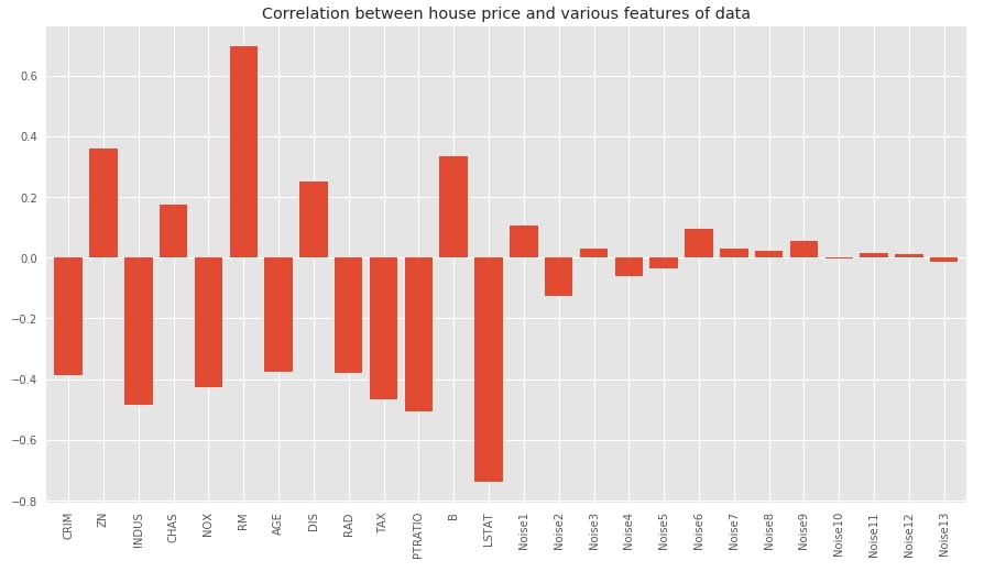
Below we have plotted bar chart showing the correlation between features of dataset and target variables. We can notice from the chart that original variables have quite a high correlation compared to noise data added later. The noise features have very little or almost no relation with the target.
with plt.style.context(('seaborn', 'ggplot')):
    plt.figure(figsize=(15,8))
    df_regression.corr()['House Price'].drop('House Price').plot(kind='bar', width=0.8,
                                                                 title="Correlation between house price and various features of data");
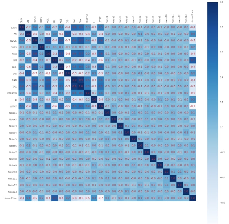
Below we have plotted heatmap showing the relationship between various features of the dataset as well as between features and target. This gives us a bigger picture giving insights about feature relations with one another.
with plt.style.context(('seaborn', 'ggplot')):
    fig = plt.figure(figsize=(18,18))
    plt.matshow(df_regression.corr().values,fignum=1, cmap = plt.cm.Blues)
    plt.xticks(range(0,27),list(boston.feature_names) + ['Noise'+str(i) for i in range(1,14)]+['House Price'], rotation='vertical')
    plt.yticks(range(0,27),list(boston.feature_names) + ['Noise'+str(i) for i in range(1,14)]+['House Price'], rotation='horizontal')
    plt.colorbar()
    plt.grid(b=False)
    for i in range(0,27):
        for j in range(0,27):
            if df_regression.corr().values[i, j] < 0:
                plt.text(i-0.4, j+0.1, '%.1f'%df_regression.corr().values[i, j], color='tab:red', fontsize=12);
            else:
                plt.text(i-0.3, j+0.1, '%.1f'%df_regression.corr().values[i, j], color='tab:red', fontsize=12);
2. Classification
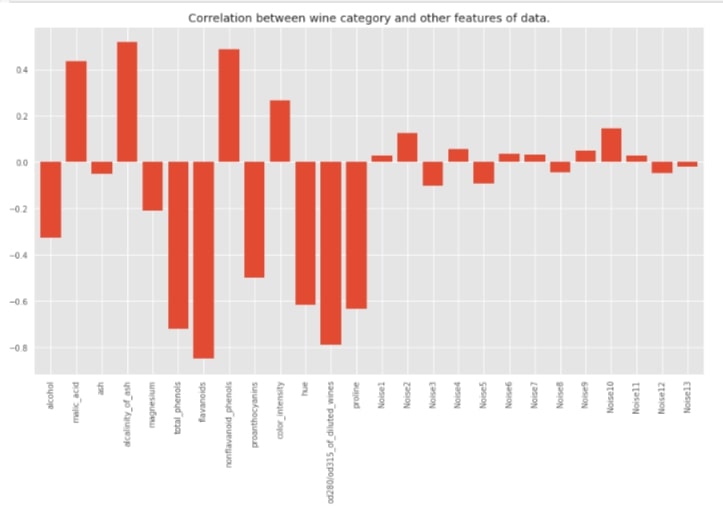
We'll now create a dataframe for the wine dataset exactly like the previous Boston housing dataset. We'll be using this dataframe for finding out the correlation between features and the target variable.
df_classif = pd.DataFrame(X_wine, columns=list(wine.feature_names) + ['Noise'+str(i) for i in range(1,14)])
df_classif['Wine Type'] = Y_wine
df_classif.head()
with plt.style.context(('seaborn', 'ggplot')):
    plt.figure(figsize=(15,8))
    df_classif.corr()['Wine Type'].drop('Wine Type').plot(kind='bar', width=0.8,
                                                          title="Correlation between wine category and other features of data.");
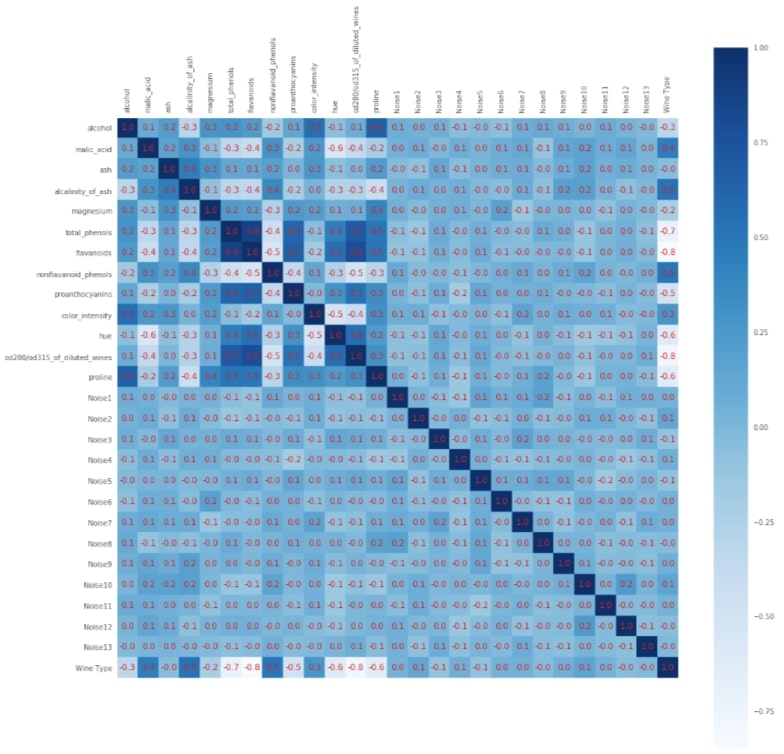
with plt.style.context(('seaborn', 'ggplot')):
    fig = plt.figure(figsize=(18,18))
    plt.matshow(df_classif.corr().values,fignum=1, cmap = plt.cm.Blues)
    plt.xticks(range(0,27),list(wine.feature_names) + ['Noise'+str(i) for i in range(1,14)]+['Wine Type'], rotation='vertical')
    plt.yticks(range(0,27),list(wine.feature_names) + ['Noise'+str(i) for i in range(1,14)]+['Wine Type'], rotation='horizontal')
    plt.colorbar()
    plt.grid(b=False)
    for i in range(0,27):
        for j in range(0,27):
            if df_classif.corr().values[i, j] < 0:
                plt.text(i-0.4, j+0.1, '%.1f'%df_classif.corr().values[i, j], color='tab:red', fontsize=12);
            else:
                plt.text(i-0.3, j+0.1, '%.1f'%df_classif.corr().values[i, j], color='tab:red', fontsize=12);
We'll now start with an explanation of various feature selection estimators available with scikit-learn and use them for classification and regression datasets to select appropriate features.
Univariate Statics 
It looks at each feature individually and selects features through the statistical test which are closely related to the target. This kind of test is known as Analysis of Variance (ANOVA). Below is a list of estimators that sklearn provides which selects features from data based on univariate statistics.
- SelectPercentile
- SelectKBest
- SelectFpr
- SelectFdr
- SelectFwe
SelectPercentile 
The SelectPercentile estimator available as a part of the feature_selection module of sklearn, let us select the percentage of highest scoring features according to univariate statistical tests.
Below are important parameters of SelectPercentile:
- score_func -It accepts callable (function). The function should accept
(features, target)as input and return two arrays (scores, p-values) or at least one array with scores for each feature. Based on these scores, features selection is made. The default value is thef_classiffunction available in thefeature_selectionmodule of sklearn. - percentile - It let us select that many percentages of features from the original feature set.
We'll now try SelectPercentile on the classification and regression datasets that we created above. We'll also check the performance of LinearRegression and LogisticRegression estimators on features that were selected by SelectPercentile. We'll plot features that were selected by SelectPercentile to check how many features it selected from original data and whether it was able to get rid of all noise features that were added to original data.
1. Classification - f_classif
Please make a note that we have tried all univariate statistics based feature selection estimators with f_classif for classification problems and f_regression for regression problems. Scikit-Learn also provides chi2 & mutual_info_classif functions for classification and mutual_info_regression for regression problems. The mutual info functions measures mutual relation between features and target variables. It then uses this information for feature selection.
from sklearn.feature_selection import f_regression, f_classif, chi2, mutual_info_classif, mutual_info_regression
from sklearn.feature_selection import SelectPercentile


print('Train/Test Sizes Before Feature Selection : ',X_train_wine.shape, X_test_wine.shape)

select_percentile_classif = SelectPercentile(score_func=f_classif, percentile=50)
select_percentile_classif.fit(X_train_wine, Y_train_wine)

X_train_selected = select_percentile_classif.transform(X_train_wine)
X_test_selected  = select_percentile_classif.transform(X_test_wine)

print('Train/Test Sizes After 50 Percentile Feature Selection: ',X_train_selected.shape, X_test_selected.shape)
from sklearn.linear_model import LogisticRegression

lr = LogisticRegression(solver='lbfgs')
lr.fit(X_train_selected, Y_train_wine)

print('Test Accuracy : ', lr.score(X_test_selected, Y_test_wine))
print('Train Accuracy : ', lr.score(X_train_selected, Y_train_wine))
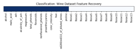
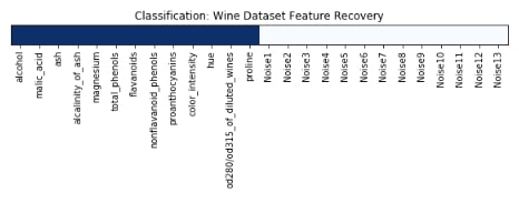
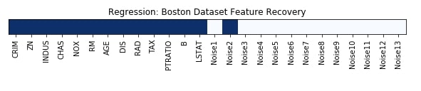
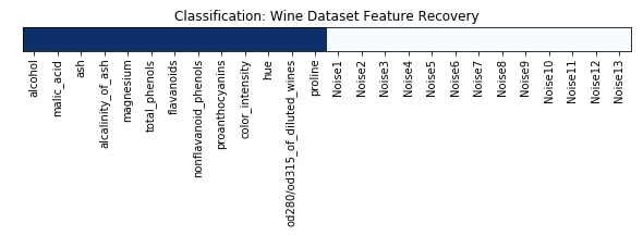
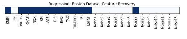
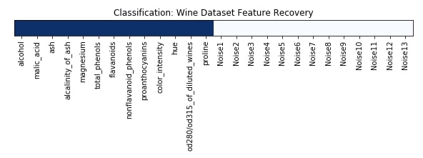
Features Recovered
The feature selection estimator has a method named get_support() which returns an array of the same size as a number of features. Its boolean array indicates whether a particular feature got selected by the feature selection estimator or not. Below we are printing values of that array as well as plotting it.
feature_selection_mask_classif = select_percentile_classif.get_support()
print('Classification Mask : ', feature_selection_mask_classif)
We have plotted features selection array which got returned by the get_support() method below. Here dark blue values represent features which got selected by model and light blue represents features which model ignored.
plt.figure(figsize=(10,11))
plt.imshow(feature_selection_mask_classif[np.newaxis,:], cmap=plt.cm.Blues)
plt.xticks(range(26), list(wine.feature_names) + ['Noise'+str(i) for i in range(1,14)], rotation='vertical')
plt.yticks([])
plt.title('Classification: Wine Dataset Feature Recovery');
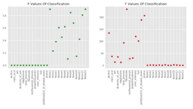
Visualising P-Values For Classification (f_classif)
sklearn provides f_classif and f_regression functions which returns F-Values and P-values for particular datasets. Lower p-values generally refer to informative features. The f-values which are generally referred to as scores of features are used by feature selection models to select features based on importance. We can notice from the below graphs that our original 13 features for classification tasks which are in beginning have low p-values compared to another 13 feature noise introduced by us later.
F_classif, p_value_classif = f_classif(X_wine, Y_wine)
with plt.style.context(('seaborn', 'ggplot')):
    plt.figure(figsize=(14,5))
    plt.subplot(121)
    plt.plot(p_value_classif, 'o', c = 'tab:green')
    plt.xticks(range(26), list(wine.feature_names) + ['Noise'+str(i) for i in range(1,14)], rotation='vertical')

    plt.title('P Values Of Classification')
    plt.subplot(122)
    plt.plot(F_classif, 'o', c = 'tab:red')
    plt.xticks(range(26), list(wine.feature_names) + ['Noise'+str(i) for i in range(1,14)], rotation='vertical')
    plt.title('F Values Of Classification');
2. Classification - chi2
Below we are using chi2 statistical estimation function as a part of SelectPercentile estimator for feature selection. Its commonly used for classification problems.
Please make a note that features passed to chi2 function should be positive. It fails if negative values are passed as a part of array. We have hence used MinMaxScaler to scale all values to be positive before passing them to chi2.
from sklearn.preprocessing import RobustScaler, StandardScaler, MinMaxScaler

print('Train/Test Sizes Before Feature Selection : ',X_train_wine.shape, X_test_wine.shape)

mms = MinMaxScaler()
X_wine_scaled = mms.fit_transform(X_wine, Y_wine)
X_train_mms = mms.transform(X_train_wine)
X_test_mms = mms.transform(X_test_wine)

select_percentile_classif_chi2 = SelectPercentile(score_func=chi2, percentile=50)
select_percentile_classif_chi2.fit(X_train_mms, Y_train_wine)

X_train_selected = select_percentile_classif_chi2.transform(X_train_mms)
X_test_selected  = select_percentile_classif_chi2.transform(X_test_mms)

print('Train/Test Sizes After 50 Percentile Feature Selection: ',X_train_selected.shape, X_test_selected.shape)
lr = LogisticRegression(solver='lbfgs')
lr.fit(X_train_selected, Y_train_wine)

print('Test Accuracy : ', lr.score(X_test_selected, Y_test_wine))
print('Train Accuracy : ', lr.score(X_train_selected, Y_train_wine))
Features Recovered
feature_selection_mask_classif_chi2 = select_percentile_classif_chi2.get_support()
print('\nClassification Mask(Chi2) : ', feature_selection_mask_classif_chi2)
plt.figure(figsize=(10,11))
plt.imshow(feature_selection_mask_classif_chi2[np.newaxis,:], cmap=plt.cm.Blues)
plt.xticks(range(26), list(wine.feature_names) + ['Noise'+str(i) for i in range(1,14)], rotation='vertical')
plt.yticks([])
plt.title('Classification: Wine Dataset Feature Recovery');

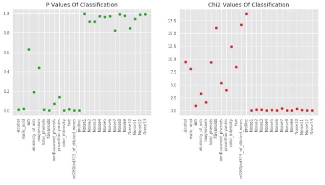
Visualising P-Values For Classification (chi2)
chi_2, p_value_classif_chi2 = chi2(X_wine_scaled, Y_wine)
with plt.style.context(('seaborn', 'ggplot')):
    plt.figure(figsize=(14,5))

    plt.subplot(121)
    plt.plot(p_value_classif_chi2, 'o', c = 'tab:green')
    plt.xticks(range(26), list(wine.feature_names) + ['Noise'+str(i) for i in range(1,14)], rotation='vertical')
    plt.title('P Values Of Classification')

    plt.subplot(122)
    plt.plot(chi_2, 'o', c = 'tab:red')
    plt.xticks(range(26), list(wine.feature_names) + ['Noise'+str(i) for i in range(1,14)], rotation='vertical')
    plt.title('Chi2 Values Of Classification');
3. Regression - f_regression
Below we are using f_regression statistical estimation function as a part of SelectPercentile estimator for feature selection. Its commonly used for regression problems.
print('Train/Test Sizes Before Feature Selection : ',X_train_boston.shape, X_test_boston.shape)

select_percentile_regression = SelectPercentile(score_func=f_regression, percentile=50)
select_percentile_regression.fit(X_train_boston, Y_train_boston)

X_train_selected = select_percentile_regression.transform(X_train_boston)
X_test_selected  = select_percentile_regression.transform(X_test_boston)

print('Train/Test Sizes After 50 Percentile Feature Selection: ',X_train_selected.shape, X_test_selected.shape)
from sklearn.linear_model import LinearRegression

lr = LinearRegression()
lr.fit(X_train_selected, Y_train_boston)

print('Test R^2 Score : ', lr.score(X_test_selected, Y_test_boston))
print('Train R^2 Score : ', lr.score(X_train_selected, Y_train_boston))
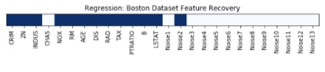
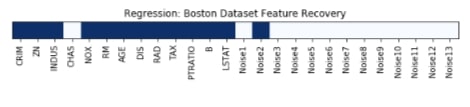
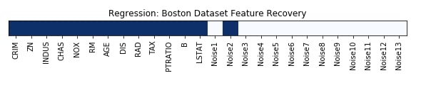
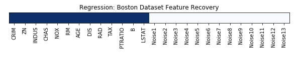
Features Recovered
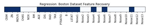
feature_selection_mask_regression = select_percentile_regression.get_support()
print('\nRegression Mask : ',feature_selection_mask_regression)
plt.figure(figsize=(10,11))
plt.imshow(feature_selection_mask_regression[np.newaxis,:], cmap=plt.cm.Blues)
plt.xticks(range(26), list(boston.feature_names) + ['Noise'+str(i) for i in range(1,14)], rotation='vertical')
plt.yticks([])
plt.title('Regression: Boston Dataset Feature Recovery');
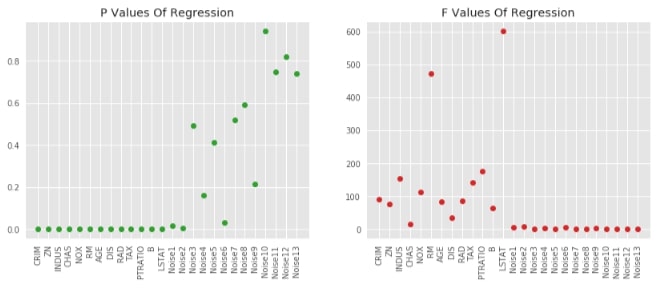
Visualising P-Values For Regression (f_regression)
F_regression, p_value_regression = f_regression(X_boston, Y_boston)
with plt.style.context(('seaborn', 'ggplot')):
    plt.figure(figsize=(14,5))
    plt.subplot(121)

    plt.plot(p_value_regression, 'o', c = 'tab:green')
    plt.xticks(range(26), list(boston.feature_names) + ['Noise'+str(i) for i in range(1,14)], rotation='vertical')
    plt.title('P Values Of Regression')

    plt.subplot(122)
    plt.plot(F_regression, 'o', c = 'tab:red')
    plt.xticks(range(26), list(boston.feature_names) + ['Noise'+str(i) for i in range(1,14)], rotation='vertical')
    plt.title('F Values Of Regression');
SelectKBest 
Sklearn provides SelectKBest estimator as a part of the feature_selection module which lets us select K best features based on scores from univariate statistical functions.
Below are important parameters of SelectKBest:
- score_func -It accepts callable (function). The function should accept
(features, target)as input and return two arrays (scores, p-values) or at least one array with scores for each feature. Based on these scores, features selection is made. The default value is thef_classiffunction available in thefeature_selectionmodule of sklearn. - k - It accepts int or
'all'as values. We can number of features to select to it as an integer.
We'll now try SelectKBest on the classification and regression datasets that we created above. We'll also check the performance of LinearRegression and LogisticRegression estimators on features that were selected by SelectKBest. We'll plot features that were selected by SelectKBest to check how many features it selected from original data and whether it was able to get rid of all noise features that were added to original data.
1. Classification
from sklearn.feature_selection import SelectKBest

print('Train/Test Sizes Before Feature Selection : ',X_train_wine.shape, X_test_wine.shape)

select_k_best_classif = SelectKBest(score_func=f_classif, k=X_wine.shape[1]//2)
select_k_best_classif.fit(X_train_wine, Y_train_wine)

X_train_selected = select_k_best_classif.transform(X_train_wine)
X_test_selected  = select_k_best_classif.transform(X_test_wine)

print('Train/Test Sizes After 50 Percentile Feature Selection: ', X_train_selected.shape, X_test_selected.shape)
lr = LogisticRegression(solver='lbfgs')
lr.fit(X_train_selected, Y_train_wine)

print('Test Accuracy : ', lr.score(X_test_selected, Y_test_wine))
print('Train Accuracy : ', lr.score(X_train_selected, Y_train_wine))
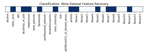
Features Recovered
feature_selection_mask_classif = select_k_best_classif.get_support()
print('Classification Mask : ', feature_selection_mask_classif)
plt.figure(figsize=(10,8))

plt.imshow(feature_selection_mask_classif[np.newaxis,:], cmap=plt.cm.Blues)
plt.xticks(range(26), list(wine.feature_names) + ['Noise'+str(i) for i in range(1,14)], rotation='vertical')
plt.yticks([])
plt.title('Classification: Wine Dataset Feature Recovery');
2. Regression
print('Train/Test Sizes Before Feature Selection : ',X_train_boston.shape, X_test_boston.shape)

select_k_best_regressor = SelectKBest(score_func=f_regression, k=X_boston.shape[1]//2)
select_k_best_regressor.fit(X_train_boston, Y_train_boston)

X_train_selected = select_k_best_regressor.transform(X_train_boston)
X_test_selected  = select_k_best_regressor.transform(X_test_boston)

print('Train/Test Sizes After 50 Percentile Feature Selection: ', X_train_selected.shape, X_test_selected.shape)
lr = LinearRegression()
lr.fit(X_train_selected, Y_train_boston)
print('Test R^2 Score: ', lr.score(X_test_selected, Y_test_boston))
print('Train R^2 Score : ', lr.score(X_train_selected, Y_train_boston))
Features Recovered
feature_selection_mask_regression = select_k_best_regressor.get_support()
print('Regression Mask : ', feature_selection_mask_regression)
plt.figure(figsize=(10,8))

plt.imshow(feature_selection_mask_regression[np.newaxis,:], cmap=plt.cm.Blues)
plt.xticks(range(26), list(boston.feature_names) + ['Noise'+str(i) for i in range(1,14)], rotation='vertical')
plt.yticks([])
plt.title('Regression: Boston Dataset Feature Recovery');
SelectFpr 
SelectFpr estimator is provided by the feature_selection module of sklearn. It let us select features based on the false-positive rate. It tries to control the total amount of false predictions per class.
Below we have given important attributes of SelectFpr estimator:
- score_func -It accepts callable (function). The function should accept
(features, target)as input and return two arrays (scores, p-values) or at least one array with scores for each feature. Based on these scores, features selection is made. The default value is thef_classiffunction available in thefeature_selectionmodule of sklearn. - alpha - It let us specify
p-value. All the features whose p-value is below this will be selected. The default value is0.05.
We'll now try SelectFpr on the classification and regression datasets that we created above. We'll also check the performance of LinearRegression and LogisticRegression estimators on features that were selected by SelectFpr. We'll plot features that were selected by SelectFpr to check how many features it selected from original data and whether it was able to get rid of all noise features that were added to original data.
1. Classification
from sklearn.feature_selection import SelectFpr

print('Train/Test Sizes Before Feature Selection : ',X_train_wine.shape, X_test_wine.shape)

select_fpr_classif = SelectFpr(score_func=f_classif)
select_fpr_classif.fit(X_train_wine, Y_train_wine)

X_train_selected = select_fpr_classif.transform(X_train_wine)
X_test_selected  = select_fpr_classif.transform(X_test_wine)

print('Train/Test Sizes After Feature Selection: ', X_train_selected.shape, X_test_selected.shape)
lr = LogisticRegression(solver='lbfgs')
lr.fit(X_train_selected, Y_train_wine)

print('Test Accuracy : ', lr.score(X_test_selected, Y_test_wine))
print('Train Accuracy : ', lr.score(X_train_selected, Y_train_wine))
Features Recovered
feature_selection_mask_classif = select_fpr_classif.get_support()
print('Classification Mask : ', feature_selection_mask_classif)
plt.figure(figsize=(10,8))

plt.imshow(feature_selection_mask_classif[np.newaxis,:], cmap=plt.cm.Blues)
plt.xticks(range(26), list(wine.feature_names) + ['Noise'+str(i) for i in range(1,14)], rotation='vertical')
plt.yticks([])
plt.title('Classification: Wine Dataset Feature Recovery');
2. Regression
print('Train/Test Sizes Before Feature Selection : ',X_train_boston.shape, X_test_boston.shape)

select_fpr_regressor = SelectFpr(score_func=f_regression)
select_fpr_regressor.fit(X_train_boston, Y_train_boston)

X_train_selected = select_fpr_regressor.transform(X_train_boston)
X_test_selected  = select_fpr_regressor.transform(X_test_boston)

print('Train/Test Sizes After 50 Percentile Feature Selection: ', X_train_selected.shape, X_test_selected.shape)
lr = LinearRegression()
lr.fit(X_train_selected, Y_train_boston)
print('Test R^2 Score: ', lr.score(X_test_selected, Y_test_boston))
print('Train R^2 Score : ', lr.score(X_train_selected, Y_train_boston))
Features Recovered
feature_selection_mask_regression = select_fpr_regressor.get_support()
print('Regression Mask : ', feature_selection_mask_regression)
plt.figure(figsize=(10,8))

plt.imshow(feature_selection_mask_regression[np.newaxis,:], cmap=plt.cm.Blues)
plt.xticks(range(26), list(boston.feature_names) + ['Noise'+str(i) for i in range(1,14)], rotation='vertical')
plt.yticks([])
plt.title('Regression: Boston Dataset Feature Recovery');
SelectFdr 
SelectFdr estimator is provided by the feature_selection module of sklearn. It let us select features based on false discovery rate. It tries to control the total amount of false predictions per class.
Below we have given important attributes of SelectFpr estimator:
- score_func -It accepts callable (function). The function should accept
(features, target)as input and return two arrays (scores, p-values) or at least one array with scores for each feature. Based on these scores, features selection is made. The default value is thef_classiffunction available in thefeature_selectionmodule of sklearn. - alpha - It let us specify highest uncorrected
p-valuefor features. The default value is0.05.
We'll now try SelectFdr on the classification and regression datasets that we created above. We'll also check the performance of LinearRegression and LogisticRegression estimators on features that were selected by SelectFdr. We'll plot features that were selected by SelectFdr to check how many features it selected from original data and whether it was able to get rid of all noise features that were added to original data.
1. Classification
from sklearn.feature_selection import SelectFdr

print('Train/Test Sizes Before Feature Selection : ',X_train_wine.shape, X_test_wine.shape)

select_fdr_classif = SelectFdr(score_func=f_classif)
select_fdr_classif.fit(X_train_wine, Y_train_wine)

X_train_selected = select_fdr_classif.transform(X_train_wine)
X_test_selected  = select_fdr_classif.transform(X_test_wine)

print('Train/Test Sizes After Feature Selection: ', X_train_selected.shape, X_test_selected.shape)
lr = LogisticRegression(solver='lbfgs')
lr.fit(X_train_selected, Y_train_wine)

print('Test Accuracy : ', lr.score(X_test_selected, Y_test_wine))
print('Train Accuracy : ', lr.score(X_train_selected, Y_train_wine))
Features Recovered
feature_selection_mask_classif = select_fdr_classif.get_support()
print('Classification Mask : ', feature_selection_mask_classif)
plt.figure(figsize=(10,8))

plt.imshow(feature_selection_mask_classif[np.newaxis,:], cmap=plt.cm.Blues)
plt.xticks(range(26), list(wine.feature_names) + ['Noise'+str(i) for i in range(1,14)], rotation='vertical')
plt.yticks([])
plt.title('Classification: Wine Dataset Feature Recovery');
2. Regression
print('Train/Test Sizes Before Feature Selection : ',X_train_boston.shape, X_test_boston.shape)

select_fdr_regressor = SelectFdr(score_func=f_regression)
select_fdr_regressor.fit(X_train_boston, Y_train_boston)

X_train_selected = select_fdr_regressor.transform(X_train_boston)
X_test_selected  = select_fdr_regressor.transform(X_test_boston)

print('Train/Test Sizes After 50 Percentile Feature Selection: ', X_train_selected.shape, X_test_selected.shape)
lr = LinearRegression()
lr.fit(X_train_selected, Y_train_boston)
print('Test R^2 Score: ', lr.score(X_test_selected, Y_test_boston))
print('Train R^2 Score : ', lr.score(X_train_selected, Y_train_boston))
Features Recovered
feature_selection_mask_regression = select_fdr_regressor.get_support()
print('Regression Mask : ', feature_selection_mask_regression)
plt.figure(figsize=(10,8))

plt.imshow(feature_selection_mask_regression[np.newaxis,:], cmap=plt.cm.Blues)
plt.xticks(range(26), list(boston.feature_names) + ['Noise'+str(i) for i in range(1,14)], rotation='vertical')
plt.yticks([])
plt.title('Regression: Boston Dataset Feature Recovery');
SelectFwe 
SelectFwe estimator is provided by the feature_selection module of sklearn. It let us select features based on the family-wise error rate.
Below we have given important attributes of SelectFwe estimator:
- score_func -It accepts callable (function). The function should accept
(features, target)as input and return two arrays (scores, p-values) or at least one array with scores for each feature. Based on these scores, features selection is made. The default value is thef_classiffunction available in thefeature_selectionmodule of sklearn. - alpha - It let us specify highest uncorrected
p-valuefor features to keep. The default value is0.05.
We'll now try SelectFwe on the classification and regression datasets that we created above. We'll also check the performance of LinearRegression and LogisticRegression estimators on features that were selected by SelectFwe. We'll plot features that were selected by SelectFwe to check how many features it selected from original data and whether it was able to get rid of all noise features that were added to original data.
1. Classification
from sklearn.feature_selection import SelectFwe

print('Train/Test Sizes Before Feature Selection : ',X_train_wine.shape, X_test_wine.shape)

select_fwe_classif = SelectFwe(score_func=f_classif)
select_fwe_classif.fit(X_train_wine, Y_train_wine)

X_train_selected = select_fwe_classif.transform(X_train_wine)
X_test_selected  = select_fwe_classif.transform(X_test_wine)

print('Train/Test Sizes After Feature Selection: ', X_train_selected.shape, X_test_selected.shape)
lr = LogisticRegression(solver='lbfgs')
lr.fit(X_train_selected, Y_train_wine)

print('Test Accuracy : ', lr.score(X_test_selected, Y_test_wine))
print('Train Accuracy : ', lr.score(X_train_selected, Y_train_wine))
Features Recovered
feature_selection_mask_classif = select_fwe_classif.get_support()
print('Classification Mask : ', feature_selection_mask_classif)
plt.figure(figsize=(10,8))

plt.imshow(feature_selection_mask_classif[np.newaxis,:], cmap=plt.cm.Blues)
plt.xticks(range(26), list(wine.feature_names) + ['Noise'+str(i) for i in range(1,14)], rotation='vertical')
plt.yticks([])
plt.title('Classification: Wine Dataset Feature Recovery');

2. Regression
print('Train/Test Sizes Before Feature Selection : ',X_train_boston.shape, X_test_boston.shape)

select_fwe_regressor = SelectFwe(score_func=f_regression)
select_fwe_regressor.fit(X_train_boston, Y_train_boston)

X_train_selected = select_fwe_regressor.transform(X_train_boston)
X_test_selected  = select_fwe_regressor.transform(X_test_boston)

print('Train/Test Sizes After 50 Percentile Feature Selection: ', X_train_selected.shape, X_test_selected.shape)
lr = LinearRegression()
lr.fit(X_train_selected, Y_train_boston)
print('Test R^2 Score: ', lr.score(X_test_selected, Y_test_boston))
print('Train R^2 Score : ', lr.score(X_train_selected, Y_train_boston))
Features Recovered
feature_selection_mask_regression = select_fwe_regressor.get_support()
print('Regression Mask : ', feature_selection_mask_regression)
plt.figure(figsize=(10,8))

plt.imshow(feature_selection_mask_regression[np.newaxis,:], cmap=plt.cm.Blues)
plt.xticks(range(26), list(boston.feature_names) + ['Noise'+str(i) for i in range(1,14)], rotation='vertical')
plt.yticks([])
plt.title('Regression: Boston Dataset Feature Recovery');
Model Based Feature Selection 
Model-based feature selection selects features from datasets by training good model like RandomForest/KnearestNeighbors and selecting features which are important from that trained model perspective. This kind of trained model will generally only keeps features that have a strong relationship with the target variable.
SelectFromModel 
Scikit-Learn provides an estimator by name SelectFromModel as a part of the feature_selection module for performing recursive feature elimination to select features. It takes other machine learning models as input based on which decision regarding feature selection will be made. It only works with a model that generates coefs_ and feature_importance_ as it selects based on values returns by these attributes of the model.
Below is a list of important parameters of SelectFromModel:
- estimator - It accepts the sklearn estimator which has
coef_andfeature_importance_attribute available once the model is trained. - threshold - It accepts
stringoffloatvalue as input. All features whose importance is greater or equal to the threshold are selected. The string value it accepts aremedianandmeanwhich will set the threshold to the median and mean ofcoef_orfeature_importance_attribute of the estimator. The default value isNonewhich will take mean of feature importance as the threshold. - max_features - It accepts
intorNone. It selects that many numbers of features which are above the threshold from total features. We can disable thethresholdparameter by setting it to-np.inf, thenSelectFromModelwill only select features specified asmax_features. - prefit - It accepts boolean value. If set to
Truethen we can pass already trained model toSelectFromModel.
We'll now try SelectFromModel on the classification and regression datasets that we created above. We'll also check the performance of LinearRegression and LogisticRegression estimators on features that were selected by SelectFromModel. We'll plot features that were selected by SelectFromModel to check how many features it selected from original data and whether it was able to get rid of all noise features that were added to original data.
1. Classification
from sklearn.feature_selection import SelectFromModel
from sklearn.ensemble import GradientBoostingClassifier, RandomForestClassifier, ExtraTreesClassifier
from sklearn.tree import DecisionTreeClassifier

print('Train/Test Sizes Before Feature Selection : ',X_train_wine.shape, X_test_wine.shape)

select_from_model_classif = SelectFromModel(ExtraTreesClassifier(max_depth=6, n_estimators=200, random_state=1), threshold='median')
select_from_model_classif.fit(X_train_wine, Y_train_wine)

X_train_selected = select_from_model_classif.transform(X_train_wine)
X_test_selected  = select_from_model_classif.transform(X_test_wine)

print('Train/Test Sizes After 50 Percentile Feature Selection: ', X_train_selected.shape, X_test_selected.shape)
lr = LogisticRegression(solver='lbfgs')
lr.fit(X_train_selected, Y_train_wine)
print('Test Accuracy : ', lr.score(X_test_selected, Y_test_wine))
print('Train Accuracy : ', lr.score(X_train_selected, Y_train_wine))
Feature Recovered
feature_selection_mask_classif = select_from_model_classif.get_support()
print('Classification Mask : ', feature_selection_mask_classif)
plt.figure(figsize=(10,8))

plt.imshow(feature_selection_mask_classif[np.newaxis,:], cmap=plt.cm.Blues)
plt.xticks(range(26), list(wine.feature_names) + ['Noise'+str(i) for i in range(1,14)], rotation='vertical')
plt.yticks([])
plt.title('Classification: Wine Dataset Feature Recovery');

2. Regression
from sklearn.ensemble import GradientBoostingRegressor, RandomForestRegressor, ExtraTreesRegressor
from sklearn.tree import DecisionTreeRegressor

X_train, X_test, Y_train, Y_test = train_test_split(X_boston, Y_boston, train_size=0.80, test_size=0.20, random_state=123)
print('Train/Test Sizes Before Feature Selection : ',X_train.shape, X_test.shape, Y_train.shape, Y_test.shape)

select_from_model_regressor = SelectFromModel(ExtraTreesRegressor(max_depth=3, n_estimators=150, random_state=1), threshold='median')
select_from_model_regressor.fit(X_train, Y_train)

X_train_selected = select_from_model_regressor.transform(X_train)
X_test_selected  = select_from_model_regressor.transform(X_test)

print('Train/Test Sizes After 50 Percentile Feature Selection: ', X_train_selected.shape, X_test_selected.shape, Y_train.shape, Y_test.shape)

lr = LinearRegression()
lr.fit(X_train_selected, Y_train)
print('Test Accuracy : ', lr.score(X_test_selected, Y_test))
print('Train Accuracy : ', lr.score(X_train_selected, Y_train))
Feature Recovered
feature_selection_mask_regression = select_from_model_regressor.get_support()
print('Regression Mask : ', feature_selection_mask_regression)
plt.figure(figsize=(10,8))

plt.imshow(feature_selection_mask_regression[np.newaxis,:], cmap=plt.cm.Blues)
plt.xticks(range(26), list(boston.feature_names) + ['Noise'+str(i) for i in range(1,14)], rotation='vertical')
plt.yticks([])
plt.title('Regression: Boston Dataset Feature Recovery');
Recursive Feature Elimination 
Recursive Feature Elimination selects all sets of features and recursively eliminates a single feature at a time. It recursively eliminates features until the desired number of features is selected.
RFE 
Scikit-Learn provides an estimator by name RFE as a part of the feature_selection module for performing recursive feature elimination to select features. It takes other machine learning models as input based on which decision regarding feature selection will be made. It only works with a model that generates coef_ and feature_importance_ as it selects based on values returned by these attributes of the model.
Below is a list of important parameters of RFE estimator:
- estimator - It accepts scikit-learn estimator which has
coef_orfeature_importance_attributes because the selection of features will be made based on these parameters. The estimator is trained and features which model thinks important are kept. - n_features_to_select - It accepts
intorNoneas value. We can specify the number of features to select from the original dataset as an integer. If we don't pass count of features to select then it'll select half of the features from the original dataset. - step - It accepts
intorfloatvalue. If an integer value greater than 1 is passed then that many features are eliminated at each iteration of RFE. If float between0-1is passed then that many percentages of features are eliminated at each iteration of RFE.
Unlike SelectFromModel which selects features by training estimator only once and selecting features, RFE trains estimator and drop features based on step parameter and then repeat the same process until n_features_to_select features are selected.
We'll now try RFE on the classification and regression datasets that we created above. We'll also check the performance of LinearRegression and LogisticRegression estimators on features that were selected by RFE. We'll plot features that were selected by RFE to check how many features it selected from original data and whether it was able to get rid of all noise features that were added to original data.
1. Classification
from sklearn.feature_selection import RFE
from sklearn.ensemble import GradientBoostingClassifier, RandomForestClassifier, ExtraTreesClassifier
from sklearn.tree import DecisionTreeClassifier

print('Train/Test Sizes Before Feature Selection : ', X_train_wine.shape, X_test_wine.shape)

rfe_classif = RFE(ExtraTreesClassifier(max_depth=6, n_estimators=200, random_state=1), n_features_to_select=13)
rfe_classif.fit(X_train_wine, Y_train_wine)

X_train_selected = rfe_classif.transform(X_train_wine)
X_test_selected  = rfe_classif.transform(X_test_wine)

print('Train/Test Sizes After 50 Percentile Feature Selection: ', X_train_selected.shape, X_test_selected.shape)
lr = LogisticRegression(solver='lbfgs')
lr.fit(X_train_selected, Y_train_wine)
print('Test Accuracy : ', lr.score(X_test_selected, Y_test_wine))
print('Train Accuracy : ', lr.score(X_train_selected, Y_train_wine))
Feature Recovered
feature_selection_mask_classif = rfe_classif.get_support()
print('Classification Mask : ', feature_selection_mask_classif)
plt.figure(figsize=(10,8))

plt.imshow(feature_selection_mask_classif[np.newaxis,:], cmap=plt.cm.Blues)
plt.xticks(range(26), list(wine.feature_names) + ['Noise'+str(i) for i in range(1,14)], rotation='vertical')
plt.yticks([])
plt.title('Classification: Wine Dataset Feature Recovery');
2. Regression
from sklearn.ensemble import GradientBoostingRegressor, RandomForestRegressor, ExtraTreesRegressor
from sklearn.tree import DecisionTreeRegressor

print('Train/Test Sizes Before Feature Selection : ',X_train_boston.shape, X_test_boston.shape)

rfe_regressor = RFE(ExtraTreesRegressor(max_depth=3, n_estimators=150, random_state=1), n_features_to_select=13)
rfe_regressor.fit(X_train_boston, Y_train_boston)

X_train_selected = rfe_regressor.transform(X_train_boston)
X_test_selected  = rfe_regressor.transform(X_test_boston)

print('Train/Test Sizes After 50 Percentile Feature Selection: ', X_train_selected.shape, X_test_selected.shape)
lr = LinearRegression()
lr.fit(X_train_selected, Y_train_boston)
print('Test R^2 Score: ', lr.score(X_test_selected, Y_test_boston))
print('Train R^2 Score : ', lr.score(X_train_selected, Y_train_boston))
Feature Recovered
feature_selection_mask_regression = rfe_regressor.get_support()
print('Regression Mask : ', feature_selection_mask_regression)
plt.figure(figsize=(10,8))

plt.imshow(feature_selection_mask_regression[np.newaxis,:], cmap=plt.cm.Blues)
plt.xticks(range(26), list(boston.feature_names) + ['Noise'+str(i) for i in range(1,14)], rotation='vertical')
plt.yticks([])
plt.title('Regression: Boston Dataset Feature Recovery');
VarianceThreshold 
The VarianceThreshold feature selection estimator as its name suggests selects only features that meet a particular threshold. It removes features whose variance does not meet that defined threshold. VarianceThereshold estimator accepts only 1 parameter threshold. If we do not provide any threshold values then it removes features which do not have variance (meaning all values are same).
We'll now try VarianceThereshold on the classification and regression datasets that we created above. We'll also check the performance of LinearRegression and LogisticRegression estimators on features that were selected by VarianceThereshold. We'll plot features that were selected by VarianceThreshold to check how many features it selected from original data and whether it was able to get rid of all noise features that were added to original data.
1. Classification
from sklearn.feature_selection import VarianceThreshold

print('Train/Test Sizes Before Feature Selection : ',X_train_wine.shape, X_test_wine.shape)

select_var_classif = VarianceThreshold(threshold=0.99)
select_var_classif.fit(X_train_wine, Y_train_wine)

X_train_selected = select_var_classif.transform(X_train_wine)
X_test_selected  = select_var_classif.transform(X_test_wine)

print('Train/Test Sizes After Feature Selection: ', X_train_selected.shape, X_test_selected.shape)
lr = LogisticRegression(solver='lbfgs')
lr.fit(X_train_selected, Y_train_wine)
print('Test Accuracy : ', lr.score(X_test_selected, Y_test_wine))
print('Train Accuracy : ', lr.score(X_train_selected, Y_train_wine))
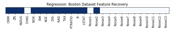
Features Recovered
feature_selection_mask_classif = select_var_classif.get_support()
print('Classification Mask : ', feature_selection_mask_classif)
plt.figure(figsize=(10,8))

plt.imshow(feature_selection_mask_classif[np.newaxis,:], cmap=plt.cm.Blues)
plt.xticks(range(26), list(wine.feature_names) + ['Noise'+str(i) for i in range(1,14)], rotation='vertical')
plt.yticks([])
plt.title('Classification: Wine Dataset Feature Recovery');
Important Attributes of VarianceThreshold
Below is a list of important features of VarianceThereshold:
- variances_ - It represents variances for each feature of the dataset.
print("Variance Size : ", select_var_classif.variances_.shape)
select_var_classif.variances_
2. Regression
print('Train/Test Sizes Before Feature Selection : ',X_train_boston.shape, X_test_boston.shape)

select_var_regressor = VarianceThreshold(threshold=0.99)
select_var_regressor.fit(X_train_boston, Y_train_boston)

X_train_selected = select_var_regressor.transform(X_train_boston)
X_test_selected  = select_var_regressor.transform(X_test_boston)

print('Train/Test Sizes After 50 Percentile Feature Selection: ', X_train_selected.shape, X_test_selected.shape)
lr = LinearRegression()
lr.fit(X_train_selected, Y_train_boston)
print('Test R^2 Score: ', lr.score(X_test_selected, Y_test_boston))
print('Train R^2 Score : ', lr.score(X_train_selected, Y_train_boston))
Features Recovered
feature_selection_mask_regression = select_var_regressor.get_support()
print('Regression Mask : ', feature_selection_mask_regression)
plt.figure(figsize=(10,8))

plt.imshow(feature_selection_mask_regression[np.newaxis,:], cmap=plt.cm.Blues)
plt.xticks(range(26), list(boston.feature_names) + ['Noise'+str(i) for i in range(1,14)], rotation='vertical')
plt.yticks([])
plt.title('Regression: Boston Dataset Feature Recovery');
This ends our small tutorial on feature selection using scikit-learn. Please feel free to let us know your views in the comments section.
References 
 Sunny Solanki
Sunny Solanki
Intro: Software Developer | Youtuber | Bonsai Enthusiast
About: Sunny Solanki holds a bachelor's degree in Information Technology (2006-2010) from L.D. College of Engineering. Post completion of his graduation, he has 8.5+ years of experience (2011-2019) in the IT Industry (TCS). His IT experience involves working on Python & Java Projects with US/Canada banking clients. Since 2020, he’s primarily concentrating on growing CoderzColumn.
His main areas of interest are AI, Machine Learning, Data Visualization, and Concurrent Programming. He has good hands-on with Python and its ecosystem libraries.
Apart from his tech life, he prefers reading biographies and autobiographies. And yes, he spends his leisure time taking care of his plants and a few pre-Bonsai trees.
Contact: sunny.2309@yahoo.in


![YouTube Subscribe]() Comfortable Learning through Video Tutorials?
Comfortable Learning through Video Tutorials?
If you are more comfortable learning through video tutorials then we would recommend that you subscribe to our YouTube channel.
![Need Help]() Stuck Somewhere? Need Help with Coding? Have Doubts About the Topic/Code?
Stuck Somewhere? Need Help with Coding? Have Doubts About the Topic/Code?
 Stuck Somewhere? Need Help with Coding? Have Doubts About the Topic/Code?
When going through coding examples, it's quite common to have doubts and errors.
If you have doubts about some code examples or are stuck somewhere when trying our code, send us an email at coderzcolumn07@gmail.com. We'll help you or point you in the direction where you can find a solution to your problem.
You can even send us a mail if you are trying something new and need guidance regarding coding. We'll try to respond as soon as possible.
![Share Views]() Want to Share Your Views? Have Any Suggestions?
Want to Share Your Views? Have Any Suggestions?
 Want to Share Your Views? Have Any Suggestions?
If you want to
- provide some suggestions on topic
- share your views
- include some details in tutorial
- suggest some new topics on which we should create tutorials/blogs
 sklearn, feature-selection