Optuna: Complete Guide to Hyperparameters Tuning / Optimization¶

Machine learning is a branch of artificial intelligence that focuses on designing algorithms that can automate a task by learning from data and experience. Machine learning algorithms are nowadays used in the majority of fields like object detection, image classification, house price prediction, email classification, and many more.

> What are Hyperparameters of ML Models?¶

Majority of machine learning algorithm has a bunch of parameters whose different values need to be tried in order to get a generalized algorithm. These parameters of the algorithms are generally referred to as hyperparameters.

Common examples of hyperparameters are penalties for an algorithm (l1 or l2 or elastic net), a number of layers for neural networks, number of epochs, batch size, activation functions, learning rate, optimization algorithms (SGD, adam, etc), loss functions, and many more.

> What is Hyperparameters Tuning?¶

When designing an ML algorithm for a task, we try different combinations of these hyperparameters to get good results. We want a generalized algorithm that is not biased towards particular set of examples and performs well with variation of examples. This process of trying different hyperparameters is commonly referred to as hyperparameters tuning or hyperparameters optimization.

> Why Grid Search is Not Enough?¶

Grid search is one Hyperparameters tuning algorithm where we try all possible combinations of hyperparameters. Trying all possible combinations of hyperparameters can take a lot of time (sometimes even days if there is a lot of data) even on powerful computers.

We need an algorithm that tries combinations that are giving good results only.

To explain with a simple example, let's consider the below image where there are two hyperparameters to tune (C and Gamma). Accuracy is displayed on left as a color bar.

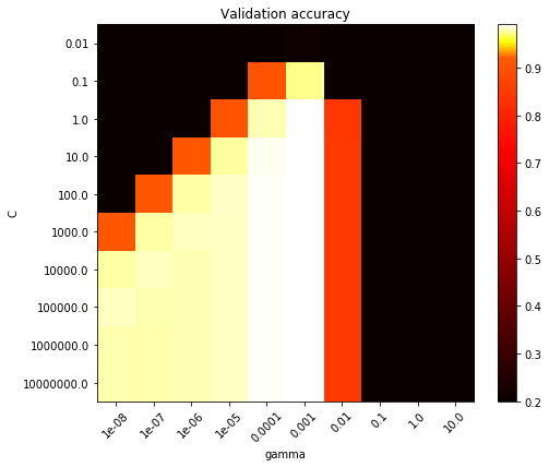
Grid search tries all combinations (Black, yellow and white area). We want an algorithm that tries few combinations from black area and deduces that they can't give good results and hence does not try more combinations from it. It'll only try combinations from white and yellow area then.

This will save us a lot of time with lots of hyperparameters.

> Which Python Libraries Performs Better Hyperparameters Tuning than Grid Search?¶

Python has libraries like Optuna, scikit-optimize, hyperopt, keras-tuner, bayes_opt, etc specifically designed for faster hyperparameters tuning.

Optuna on which we'll concentrate in this tutorial helps us find the best hyperparameters settings faster and works with a majority of current famous ML libraries like scikit-learn, xgboost, PyTorch, TensorFlow, skorch, lightGBM, Catboost, Keras, etc.

> What Can You Learn From This Article?¶

As a part of this tutorial, we have explained how to perform hyperparameters tuning of ML Models using Python library 'optuna' with simple and easy-to-understand examples. Tutorial Examples performs hyperparameters tuning of scikit-learn ML Models which are solving regression and classification tasks. Tutorial also explains various other functionalities provided by optuna like data visualization, logging, etc.

Tutorial starts by explaining hyperparameters optimization of simple line formula. The section is a bit theoretical as it has many function definitions. If you are in hurry then feel free to skip that section and go to regression or classification section. You can refer it for function definitions if you get stuck somewhere in later sections.

> How to Install 'Optuna'?¶

• PIP
  • pip install -U optuna
• Conda
  • conda install -c conda-forge optuna

Important Sections of Tutorial¶

This ends our small introduction to Optuna. We'll now start explaining the usage with examples. Our tutorial consists of the below sections.

1. Optuna Strategies for Hyperparameters Optimization
2. Steps to Use "Optuna"
3. Minimize Simple Line Formula
   • 3.1 Define Objective Function
   • 3.2 Create 'Study' Object
   • 3.3 Call "optimize()" to Perform Hyperparameters Tuning
   • 3.4 Retrieve Best Hyperparameters Combination using 'Study' Object Attributes
4. Hyperparameters Tuning Of Scikit-Learn Ridge Regression Model
   • 4.1 Load Boston Housing Dataset
   • 4.2 Divide Dataset into Train / Test Sets
   • 4.3 Define Objective Function
   • 4.4 Create Study Object and Perform Hyperparameters Tuning
   • 4.5 Print Best Hyperparameters Combination
   • 4.6 Optimize More
   • 4.7 Comparison with Grid Search
   • 4.8 Comparison with Random Search
5. Hyperparameters Tuning Of Scikit-Learn Classification (Logistic Regression) Model
   • 5.1 Load Wine Dataset
   • Remaining sections same as previous section
6. Pruning Underperforming Hyperparameters Settings Earlier
   • 6.1 Load California Housing Dataset
   • Remaining sections same as previous section
7. Data Visualizations from Optuna
8. Logging in Optuna

We'll start by importing Python library optuna.

1. Optuna Strategies for Hyperparameters Optimization ¶

Optuna overall uses the below strategy for finding the best hyperparameters combination.

1. Sampling Strategy - It uses a sampling algorithm for selecting the best hyperparameters combination from a list of all possible combinations. It concentrates on areas where hyperparameters are giving good results and ignores others resulting in time savings.
2. Pruning Strategy - It uses a pruning strategy that constantly checks for algorithm performance during training and prunes (terminates) training for particular hyperparameters combination if it's not giving good results. This also results in time-saving. (Discussed in Section 6)

2. Steps to Use "Optuna" ¶

Below we have listed steps that will be commonly followed to perform hyperparameters tuning using optuna.

1. Create an objective function.
   • This function will have logic for creating a model, training it, and evaluating it on the validation dataset. After evaluation, it should return a single value which is generally the output of the evaluation metric or loss function (accuracy, MSE, MAE, log loss, etc.) and needs to be minimized / maximized.
   • This function takes as input a single parameter which is an instance of Trial class. Trial object has details about one combination of hyperparameters with which the ML algorithm will be executed.
2. Create Study object.
3. Call optimize() method on Study by giving objective function created in the first step to find best hyperparameters combination.
   • It'll execute the objective function more than once by giving different Trial instances each having different hyperparameters combinations.

Optuna is based on the concept of Study and Trial.

• The trial is one combination of hyperparameters that will be tried with an algorithm.
• The study is the process of trying different combinations of hyperparameters to find the one combination that gives the best results. The study generally consists of many trials.

3. Minimize Simple Line Formula ¶

As a part of this section, we'll introduce how we can use Optuna to find the best parameters that can minimize the output of the simple line function.

NOTE: Please feel free to skip this section if you are in hurry and want to learn how to use Optuna with sklearn models. This section can be referred to for function definitions later. If you have enough time then it's worthwhile going through this section.

We'll be trying to minimize the line function 5x-21. We want to find the best value of x at which the output of function 5x-21 is 0. This is a simple function and we can easily calculate the output but we'll let optuna suggest values of parameter x which will minimize the function.

We'll be following the steps which we discussed in previous section.

3.1 Define Objective Function¶

We'll start by creating an objective function that takes as input instance of Trial and return the value which we want to minimize/maximize. In our case, we want to minimize the value of line function 5x-21. We have wrapped the line formula in abs function because we want to minimize the function to 0. If we don't use abs then it'll take negative values of the line formula as a minimum.

Our hyperparameter for this line formula is x. We want to find the value of x at which formula abs(5-21) is minimum. We'll be using methods of Trial instance for suggesting values of hyperparameter x for this purpose.

> Important Methods of 'Trial' Instance¶

• suggest_float(name,low,high,step=None,log=False) - This method takes as input hyperparameter name and it's low and high values as input. It then suggests float values in the range of [low, high]. We can specify step value if we want to increase the value using that step size. We can also set log parameter to True to follow a logarithmic pattern in suggesting values. Logarithmic suggestion slowly increases the value of a parameter.
• suggest_int(name,low,high,step=1,log=False) - This method works exactly like suggest_float() with only difference that it suggests integer values instead.
• suggest_uniform(name,low,high) - This method takes parameter name and low & high value of parameter. It then uniformly suggests values of parameter.
• suggest_categorical(name, choices) - This method takes as input parameter name and list of different values of that parameter that we want to try. It's generally used for categorical variables of data.

We have declared hyperparameter x using suggest_float() method inside of objective function. This will make sure that values of x are suggested as float and in the range 0-5. The new value of x will be suggested each time the objective function is called with Trial instance.

3.2 Create 'Study' Object¶

In this cell, we have created an instance of Study using create_study() method. This object will be used to try different combinations of hyperparameter combinations. In our case, different values of x will be tried by this study object.

• create_study(study_name=None,direction=None,sampler=None,pruner=None,storage=None,load_if_exists=None) - This method creates an instance of Study which will be used for optimization. It has list of optional parameters.
  • The study_name parameter accepts string specifying the name of the study.
  • The direction accepts string 'minimize' if we want to minimize the output of objective function else 'maximize'. By default, the objective function is minimized.
  • The sampler parameter accepts an instance of Sampler specifying which sampling strategy to use for selecting hyperparameter combinations. Below is a list of sampling algorithms available from Optuna.
    • TPESampler - By default this sampler will be used if none is provided. It uses a Tree-structured Parzen Estimator algorithm for selecting hyperparameter combinations.
    • CmaEsSampler - This sampler uses cmaes library for selecting hyperparameter combinations. It's implementation of covariance matrix adaptation evolution strategy (CMA-ES) algorithm.
    • NSGAIISampler - This is a multi-objective sampler based on the NSGA-II algorithm.
    • MOTPESampler - This is a multi-objective sampler based on the MOTPE algorithm.
    • GridSampler - This is the same sampler as scikit-learn's grid search will try all combinations.
    • RandomSampler - This is the same sampler as scikit-learn's random search which will randomly select few combinations.
  • The pruner parameter accepts an instance of Pruner which will be used to prune a particular trial of objective function if it's not giving good results before it completes (discussed in Section 6). Below is a list of pruners available with Optuna.
    • MedianPruner - By default this pruner will be used if none is provided. It uses the median stopping rule to prune trials.
    • NopPruner - This pruner will not perform pruning.
    • PercentilePruner - This pruner will keep the specified percentile of trials from all possible trials.
    • SuccessiveHalvingPruner - This pruner uses an asynchronous successive halving algorithm for pruning trials.
    • HyperbandPruner - It uses a hyperband algorithm for pruning.
    • ThresholdPruner - It uses a certain threshold to prune trials.
    • PatientPruner - This pruner wraps another pruner with particular tolerance and prunes trial based on it.

We'll be using the default sampler and pruner available in our examples of this tutorial.

3.3 Call "optimize()" to Perform Hyperparameters Tuning¶

Once we have created a Study object, we can instruct it to try different values of hyperparameters tuning by calling 'optimize()' method.

In our case, it'll try to find the best value of x which minimizes the line formula.

> Important Methods of 'Study' Object¶

• optimize(func,n_trials=None,storage=None,timeout=None,n_jobs=1,catch=(),show_progress_bar=False) - This method takes as input objective function and tries different combination of hyperparameters with it. It has list of important parameters.
  • The n_trials parameter accepts integer values specifying the number of trials to execute.
  • The timeout parameter accepts float value specifying the number of seconds to wait before terminating the study. It'll try different combinations until a specified amount of seconds is passed.
  • The n_jobs parameter accepts integer values specifying the number of cores/CPU to use on the computer. If we set it to -1 then it'll use all cores of the computer.
  • The catch parameter accepts a list of exceptions. The study will continue with other trials if one of the exception specified in this list happens during the execution of an objective function. By default, this list is empty which means that any exception that happened in the objective function will result in a halt of study. We can provide exceptions that we want to avoid as a part of this parameter.
  • The show_progress_bar parameter accepts a boolean value which if set to True will show the progress bar of study.
  • The storage parameter accepts database URL where trial results will be saved. This will be useful when we want to run trials in parallel on many different computers. They will communicate and divide trials using this database.

Below we have instructed Study object to try the objective function 10 times so that it'll try 10 different values of parameter x and will keep track of formula output for each try.

3.4 Retrieve Best Hyperparameters Combination using 'Study' Object Attributes¶

Study object has a list of important attributes which can be used to find out the best parameter settings and result details once the study completes executing all trials.

The best_params attribute has a dictionary specifying a value of each hyperparameter that gave the best results (minimum value of an objective function in this case).

Below we have printed the best value of x which gave the minimum value for our line formula.

The best_value attribute has a value of the best result. It'll be holding the minimum value of the line formula that we got after performing different trials.

The best_trial attribute has an instance of FrozenTrial which has details about a trial that gave the best results. It has information about a trial state which is COMPLETE in this case. The trial state can be failed or pruned as well.

The trials attribute has a list of FrozenTrial instances holding information about each individual trial and their states.

The trials_dataframe() method returns pandas dataframe summarizing all trials of study.

3.5 Further Optimization By Executing More Trials¶

We can continue our trials further by calling optimize() function. It'll try that many more trials. If we are not satisfied with the results of the initial trials then we can call optimize() again so that it tries a few more trials to improve results further.

Below we have executed 15 more trials using optimize().

Below we have printed the best parameter and the best value after trying 15 more trials.

4. Hyperparameters Tuning Of Scikit-Learn Ridge Regression Model¶

As a part of this section, we'll explain how we can use optuna with scikit-learn estimators. We'll be working on a regression problem and try to solve it using ridge regression.

We'll be using the Boston housing dataset available from scikit-learn for our purpose.

We'll also compare the results of optuna with results of grid search and random search of scikit-learn.

Below, we have imported all necessary Python libraries and functions that we'll be using throughout this section.

4.1 Load Boston Housing Dataset¶

Below we have loaded the Boston housing dataset available from scikit-learn. It has information about houses like the average number of rooms per dwelling, property tax, the crime rate in the area, etc. We'll be predicting the median value of the house in 1000 dollars. We have loaded the dataset and saved it in a data frame for display purposes.

We have stored 13 features of data into variable X and target value in variable Y.

4.2 Divide Dataset into Train / Test Sets¶

Below we have divided data into train (80%) and test (20%) sets using train_test_split() scikit-learn function.

4.3 Define Objective Function¶

Below we have declared the objective function that we'll be using for our purpose. We have declared 4 hyperparameters that we'll be optimizing.

> Hyperparameters to Tune¶

• alpha
• fit_intercept
• tol
• solver

We have used suggest_float() to suggest floating-point values for hyperparameters alpha and tol. We have used suggest_categorical() to suggest categorical values for hyperparameters fit_intercept and solver. Values of hyperparameters will be selected from ranges suggested by these methods during each trial of the optuna study.

We have then created a model with these parameters and fitted training data to it. At last, we have calculated the mean squared error (MSE) on test data and returned the value of it. We'll be minimizing this MSE during the study.

4.4 Create Study Object and Perform Hyperparameters Tuning¶

Below we have created an instance of Study and run 15 trials of the objective function that we created in the previous cell. This will try to find the best hyperparameter settings that minimize MSE on test data using TPESampler of optuna.

We have recorded execution time taken by below cell using Jupyter notebook magic command '%%time'. If you are new to magic commands of Jupyter notebook then we'll recommend going through below link in your free time.

• Jupyter Notebook Magic Commands

4.5 Print Best Hyperparameters Combination¶

Below we have printed hyperparameters combination that gave the least MSE. We have then created a ridge regression model using the best hyperparameters that we found out using optuna. We have evaluated the performance of the model on train and test set by evaluating MSE on both.

Here, we have created a ridge regression model with default parameters for comparison purposes. We have a default model with train data and then evaluated it on both train and test sets.

4.6 Optimize More¶

Now we'll optimize the objective function again for 10 trials to check whether it's improving results further or not.

This trial will work keeping 15 trials that we performed earlier as a part of this study. It'll continue to search in a direction where it had got good results (least MSE) when it ran 15 trials earlier.

Below we have printed the best parameters and MSE for that model found out after another 10 trials. We have also trained the model using these settings and evaluated it as well.

4.7 Comparison with Grid Search¶

As a part of this section, we'll compare optuna with the grid search algorithm of scikit-learn. We'll be trying the same parameter settings that we tried with optuna but we'll use grid search for training purposes.

If you are interested in learning about how to use grid search from scikit-learn then please feel free to check our tutorial on the same.

• Scikit-Learn - Hyperparameter Tuning Using GridSearch

Grid Search without Parallelization¶

Below we are trying grid search without any kind of parallelization. We have chosen the same hyperparameter ranges that we had used when using optuna.

Grid search in total below will try 3000 different combinations (25-alpha x 2-fit_intercept x 10-tol x 6-solver) of hyperparameters.

We can notice from the output that results are almost the same as that of optuna. The MSE is almost the same in both train and test sets but the time taken by grid search is a lot more than that compared to optuna.

Grid Search with Parallelization¶

Below we have tried the same grid search algorithm with parallelization to check whether there is any improvement in speed. The code has only one change compared to the previous section that we have set n_jobs parameter to -1 instructing it to use all cores of the computer.

We can notice from the output that the grid search now completes in almost half of the time compared to the previous run but still even after parallelization it took a lot more time compared to optuna.

4.8 Comparison with Random Search¶

As a part of this section, we'll be comparing the performance of optuna with that of the random search algorithm of scikit-learn for hyperparameters optimization.

If you are interested in learning about how to use random search from scikit-learn then please feel free to check our tutorial on the same.

• Scikit-Learn - Hyperparameter Tuning Using Random Search

Random Search without Parallelization¶

Below we have used random search with the same range of hyperparameters values that we had used with optuna.

We have instructed the random search algorithm to try 25 random iterations because we had run optuna earlier for 25 trials (15 first and then 10).

We can notice that random search completes quite faster compared to grid search because it tries only 25 hyperparameters combinations whereas grid search was trying 3000.

If we compare timing with optuna, the time is still quite more compared to optuna and results are almost the same.

Optuna can run still more fast if we had used parallelization with it by setting n_jobs to -1 when optimizing an objective function.

Random Search with Parallelization¶

Below we have run a random search with parallelization by setting n_jobs to -1. It now runs faster compared to the non-parallelized version but still slower compared to optuna. The results are almost the same or a little bad compared to optuna.

5. Hyperparameters Tuning Of Scikit-Learn Classification (Logistic Regression) Model¶

As a part of this section, we'll explain how we can use Optuna for classification problems.

We'll be using the wine dataset available from scikit-learn for our purpose. It has information about various ingredients of wines for three different categories of wines.

We'll be using logistic regression for explanation purposes and try to find out the best hyperparameters combination that gives the best accuracy.

5.1 Load Wine Dataset¶

Below we have loaded the wine dataset from scikit-learn. We have created a pandas data frame from wine data for the display purpose of its features and target (Wine Type) variables.

We have loaded information about wine features into a variable named X and information about wine type into a target variable named Y.

5.2 Divide Dataset into Train / Test Sets¶

Below we have divided the wine dataset into the train (80%) and test (20%) sets.

5.3 Define Objective Function¶

Below we have created an objective function for our classification problem. We'll be optimizing 5 different hyperparameters of a logistic regression model.

> Hyperparameters to Tune¶

• penalty
• tol
• C
• fit_intercept
• solver

We have used suggest_categorical() method of Trial instance for suggesting categorical values for hyperparameters penalty, fit_intercept and solver. We have used suggest_float() method for suggesting float values for hyperparameters tol and C.

We have then created logistic regression model using these hyperparameter variables, trained the model on train data and evaluated it on test data.

The evaluation will find out accuracy in this case which will tell us how many percent of test labels our model predicted correctly.

5.4 Create Study Object and Perform Hyperparameters Tuning¶

Below we have created an instance of Study with the name LogisticRegression. The optimization direction is to maximize this time because we want to maximize accuracy.

The default value of parameter direction is minimize which will minimize the output of an objective function. It was used during the regression section where we wanted to minimize MSE.

We have then used the study object and instructed it to run the objective function for 15 trials with different hyperparameter combinations.

5.5 Print Best Hyperparameters Combination¶

Below we have printed the best hyperparameters settings which gave the best accuracy on train data.

Below we have created a logistic regression model with the best parameters that we found using optuna. We have then trained it and evaluated it on train and test datasets.

5.6 Optimize More¶

Below we have instructed the study object to optimize the objective function for 10 more trials to check whether it's improving the results further or not.

We have then printed the results after another 10 trials and the results are almost the same.

5.7 Comparison with Grid Search¶

As a part of this section, we are comparing the grid search algorithm with optuna. We are trying the same ranges for each hyperparameter that we tried when using optuna.

We can notice after training and evaluation that results are almost the same but the time taken by grid search is a lot more compared to optuna.

5.8 Comparison with Random Search¶

Below we have compared a random search algorithm with optuna. We have run a random search algorithm for 25 iterations.

We can come to the conclusion that optuna finds out the best hyperparameters combination in quite less time compared to random search and grid search.

This can increase the productivity of ml practitioners a lot as it'll save time which could have been wasted in trying all possible settings rather than concentrating on ones that are giving good and ignoring others.

6. Pruning Under Performing Hyperparameters Settings Earlier ¶

As a part of this section, we'll explain how we can instruct Optuna to prune trials that are not performing well during the study process earlier.

We'll be using the California housing dataset available from scikit-learn as a part of this section. We'll be training a dataset in batches on a multi-layer perceptron algorithm available from scikit-learn.

> Why Prune Trial Earlier?¶

Typical machine learning algorithm deals with a lot of data in which case training does not complete in one go.

Real-world problems generally have a lot of data and the training process consists of going through batches of samples of data. It goes through the total data in batches to cover the total dataset.

Many neural networks even go through a dataset more than once during the training process.

When going through data in batches or even looping through the same data more than once during the particular trial of study, we can check the performance of a model on set aside validation or test set.

If it's not performing well then it can be pruned before it completes to save time and resources for other trials of the study process. Whether to prune a particular trial or not is decided by the internal pruning algorithm of Optuna.

6.1 Load California Housing Dataset¶

California housing dataset has information about houses (average bedrooms, the population of an area, house age, etc) in California and their median house price. The median house price will be the target variable that our ML algorithm will be predicting. It'll be a regression problem.

Below we have loaded the California housing dataset which is available from scikit-learn. It's a big dataset compared to our previous datasets. It has around 20k+ entries.

We have stored the dataset in a pandas dataframe for display purposes. We have stored housing features in variable X and our target variable (median house price) in variable Y.

6.2 Divide Dataset into Train / Test Sets¶

We have then divided the dataset into training (90%) and test (10%) sets as usual.

Below we have reshaped our training and test dataset so that it has now entries in batches of samples. Each entry is a batch of 16 samples of data. The ML model will loop through training data in batches where 16 samples will be fed to it for training each time.

6.3 Define Objective Function¶

Below we have created an objective function that we'll be using for our purpose. We'll be optimizing the values of the below hyperparameters of the model.

> Hyperparameters to Tune¶

• hidden_layer_sizes
• activation
• learning_rate
• learning_rate_init

Our objective function uses suggest_categorical() method of Trial instance for suggesting categorical values for hyperparameters hidden_layer_sizes, activation and learning_rate. We have used suggest_float() method for suggesting float values for hyperparameter learning_rate_init.

After that, we have initialized model with these parameters.

The training process this time consists of a loop where we go through training data and each time partially fit a model to a single batch of training data.

> How to Prune Under Performing Trial?¶

In order to prune underperforming trials, we have introduced few extra lines of code.

We are calling report() method of Trial instance which takes as input value which we are optimizing and number inside of our training loop.

Then we have put if condition which checks whether this particular trial should be pruned using should_prune() method of Trial instance.

If this method returns True then we raise TrialPruned() which will raise an exception. This will inform Study instance that we should prune this trial and should not train it more.

This will result in saving of time and resources which would have been wasted behind this trial which would have resulted in underperformed results.

The default pruning algorithm of the study instance is MedianPruner which decides whether to prune a particular trial or not.

Based on the decision taken by this algorithm, should_prune() method returns True or False.

The MedianPruner algorithm takes decisions based on MSE values that we reported through various calls of report() method during the training process.

6.4 Create Study Object and Perform Hyperparameters Tuning¶

Below we have created an instance of Study for trying various trials. We are then running 15 different trials to optimize the output (MSE on test dataset) of the objective function.

This time, we can notice from the output that few of the trials are pruned by the algorithm during a study which it thinks would not have resulted in a good performance.

6.5 Print Best Hyperparameters Combination¶

Below we have printed the best parameter settings and the least MSE that we got using those parameters.

Below we have printed the count of total trials, trials that were pruned, and trials that were completed successfully. We have used the state of the trial to determine whether they completed or got pruned. We can notice that 10 trials were pruned out of a total of 15 trials.

Below we have trained multilayer perceptron with the best parameter settings that we got through optuna. We are then evaluating its performance on the train and test dataset by calculating MSE on both.

6.6 Optimize More¶

Below we have instructed the study instance to try 5 more trials to optimize an objective function. We are doing this to check whether it's able to find hyperparameters combination which can give better results than we got during our earlier 15 trials.

Below we have printed the best hyperparameter settings as usual. Then we have again trained the model with the best hyperparameters settings that we got through optuna for verification purposes.

7. Data Visualizations ¶

As a part of this section, we'll be exploring various visualizations available through Optuna which can help us make better decisions. It gives us inside into various hyperparameters and their impact on model performance.

We'll start by checking whether visualization support is available or not using is_available() function. It checks whether proper versions of plotly and matplotlib are available or not for creating visualizations.

7.1 Optimization History Plot¶

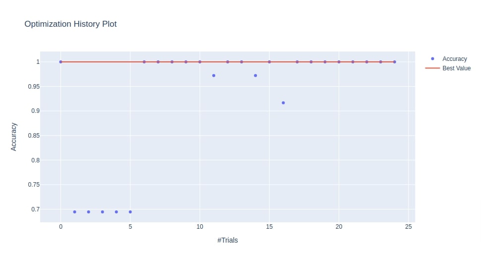
The first chart that we'll introduce is the optimization history chart. It plots the number of trials that we tried for finding the best hyperparameters combination on the Y-axis and an objective value that we got for each trial on the Y-axis.

We can use this chart to check whether hyperparameters optimization is going in the right direction or not.

• plot_optimization_history(study,target_name='Objective Value') - This function takes as input Study object and plots optimization history chart using plotly. We can give name of objective value which we were trying to minimize/maximize as the value of parameter target_name.

Below we have plotted the optimization history chart using the study object that we created during the classification section of this tutorial.

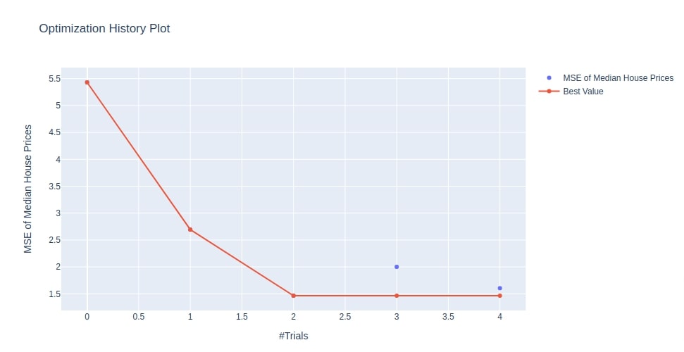
Below we have plotted the optimization history chart using the study object that we created in the multi-layer perceptron section. We can notice from the output that the value of MSE is decreasing with an increase in trials. This confirms that Optuna was looking for a hyperparameters combination in the right direction.

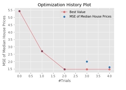
Below we have plotted an optimization history plot using matplotlib. Optuna provides us a majority of charts with matplotlib as backend as well.

7.2 Parameter Importance Plot¶

The second chart that we'll plot is a bar chart representing the hyperparameter importance of hyperparameters whose combinations were tried during the study process. This can help us understand which hyperparameters are contributing more towards minimizing/maximizing objective value.

• plot_param_importances(study, target_name='Objective Value') - This function takes as input Study object and plots bar chart of hyperparameters importance using it.

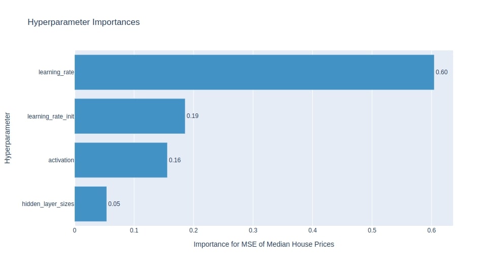
Below we have plotted hyperparameters importance chart using study object from multi-layer perceptron model section. We can notice that Optuna thinks that learning_rate is most important parameter to optimize followed by learning_rate_init, activation and hidden_layer_sizes.

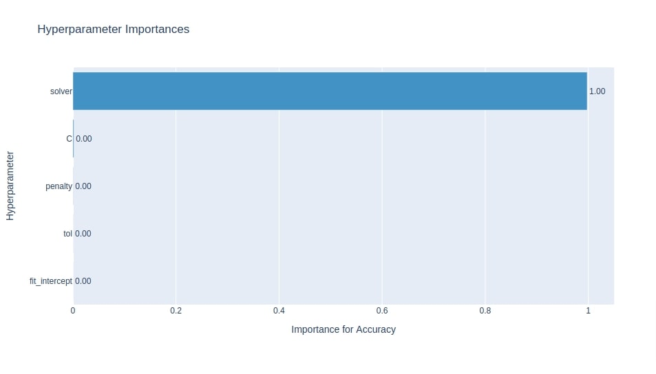
Below we have plotted hyperparameters importance chart using study object from the classification section. It seems that solver is the most important hyperparameter to tune from a chart.

7.3 HyperParameters Relationship Contour Plot¶

As a part of this section, we'll introduce a contour chart of the relationship between hyperparameters. It shows a relationship between different combinations of hyperparameters and objective value for those combinations as a contour plot.

• plot_contour(study,params=None,target_name='Objective Value') - This function takes as input study object and returns contour chart showing relationship between all combinations of hyperparameters. We can provide params parameter with a list of hyperparameters between which we want to see the relationship.

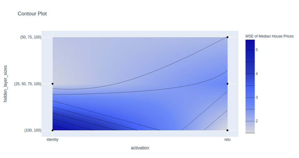
Below we have plotted contour plot using study object from multi layer perceptron section. We have plotted relationship between hyperparameters hidden_layer_sizes and activation. We can notice from the chart that value of objective function is less where hidden_layer_sizes is set to (50,75,100) and activation is set to identity.

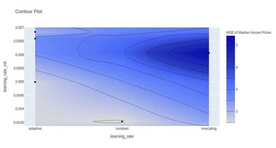
Below we have plotted another contour chart showing the relationship between learning_rate and learning_rate_init.

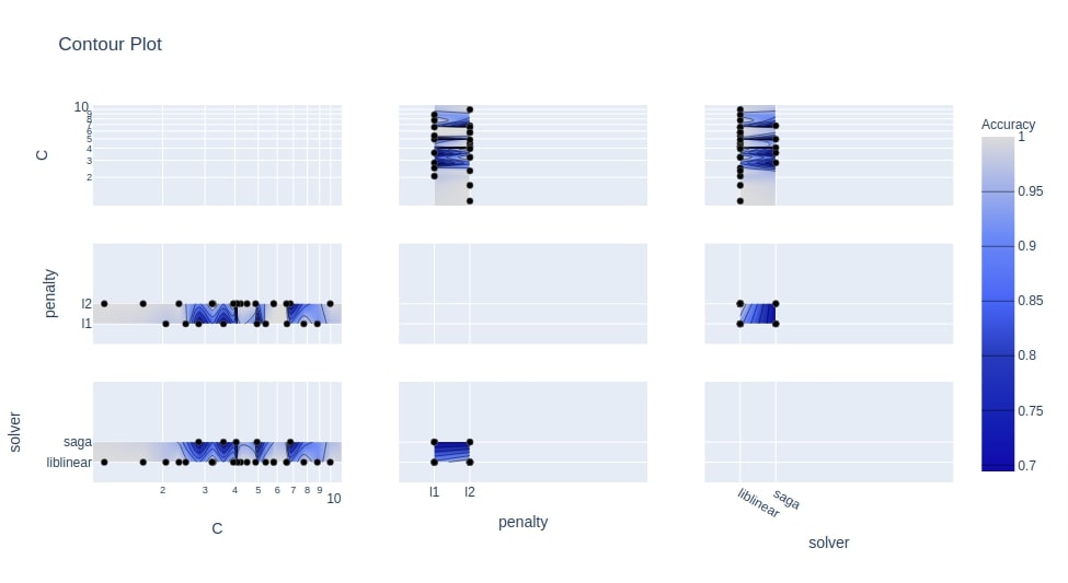
Below we have plotted our third contour chart using the study object from the classification section. We have used 3 hyperparameters (penalty, C, and solver) this time. This will create a plot with 9 contour charts where each contour chart will be showing the relationship between 2 hyperparameters.

7.4 HyperParameters Combinations and Objective Value Relationship Parallel Coordinates Plot¶

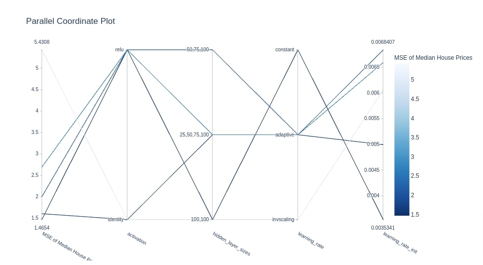
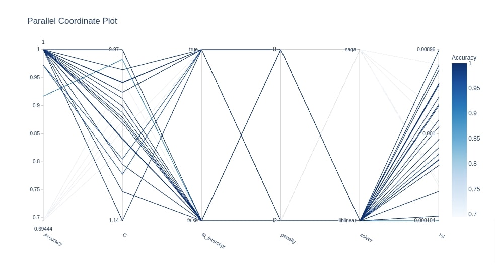
As part of this section, we'll introduce parallel coordinates chart of parameter combinations that leads to a particular value of an objective function.

The parallel coordinates chart has a single vertical line for each hyperparameter that we have tried using optuna.

The vertical lines will have different values for those parameters.

Then there will be lines connecting various values of these hyperparameters showing one combinations of these hyperparameters.

The color of the line will be based on colormap which represents an objective value that we get using those combinations of hyperparameters. The first vertical line will be representing actual values of the objective function that we were trying to minimize/maximize.

Optuna provides plot_parallel_coordinate() function for this purpose.

• plot_parallel_coordinate(study, target_name='Objective Value') - This function takes as input Study instance and creates parallel coordinates chart showing relationship between hyperparameters combination and objective value.

Below we have created parallel coordinates plot using our Study instance from the multi-layer perceptron section. We had minimized the MSE of median house prices in that section.

We can notice below in parallel coordinates chart showing different combinations of hyperparameters and their relationship with MSE.

Below we have created another parallel coordinates chart using Study object from the classification section.

7.5 HyperParameters Combination and Objective Value Relationship Slice Plot¶

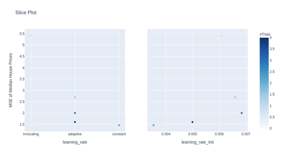
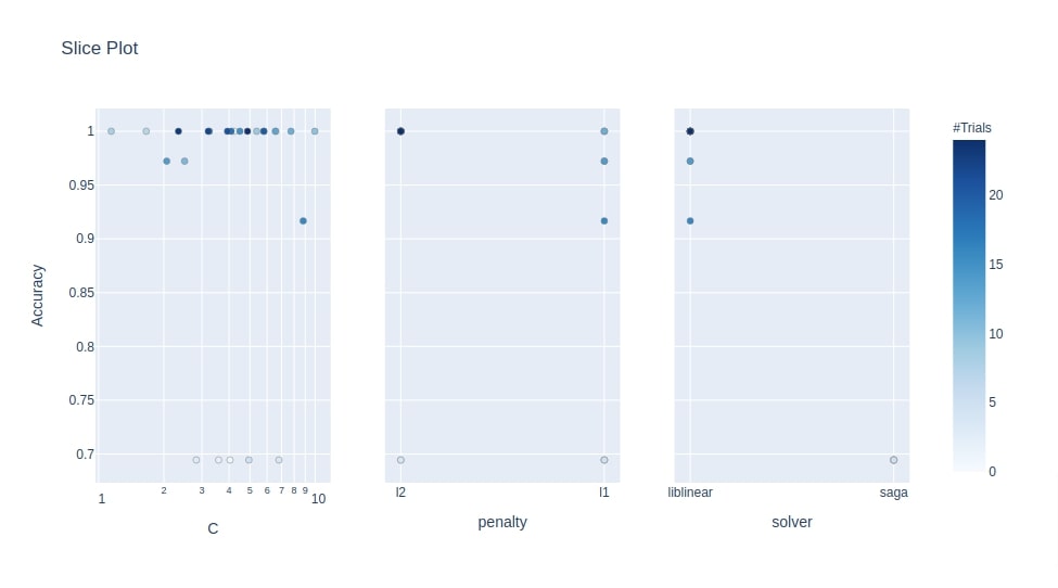
As a part of this section, we'll introduce a slice chart that shows the relationship between hyperparameter value and objective value.

It has a hyperparameter value on X-axis and an objective value on Y-axis.

We have then dots for different combinations and the opacity of that dot represents a number of trials taken to reach that objective value with that hyperparameter value of the ML model.

Optuna provides plot_slice() function for this purpose.

• plot_slice(study,params=None,target_name=None) - This function takes as input Study instance and list of hyperparameter names and then creates slice plot from it. The slice plot consists of a list of charts where an individual chart represents the relationship between one hyperparameter and the objective value.

Below we have created a slice plot from Study object of the multi-layer perceptron section. We have created a slice plot of hyperparameters learning_rate and learning_rate_init.

We can notice from dot opacity that how many trials it took for that value of hyperparameter to reach the value of MSE on the Y-axis.

Below we have created a slice plot using Study instance of the classification section. We have included hyperparameters penalty, C, and solver in the chart. It shows how many trials were taken by a particular value of hyperparameter to get particular accuracy.

7.6 Intermediate Values of Trials¶

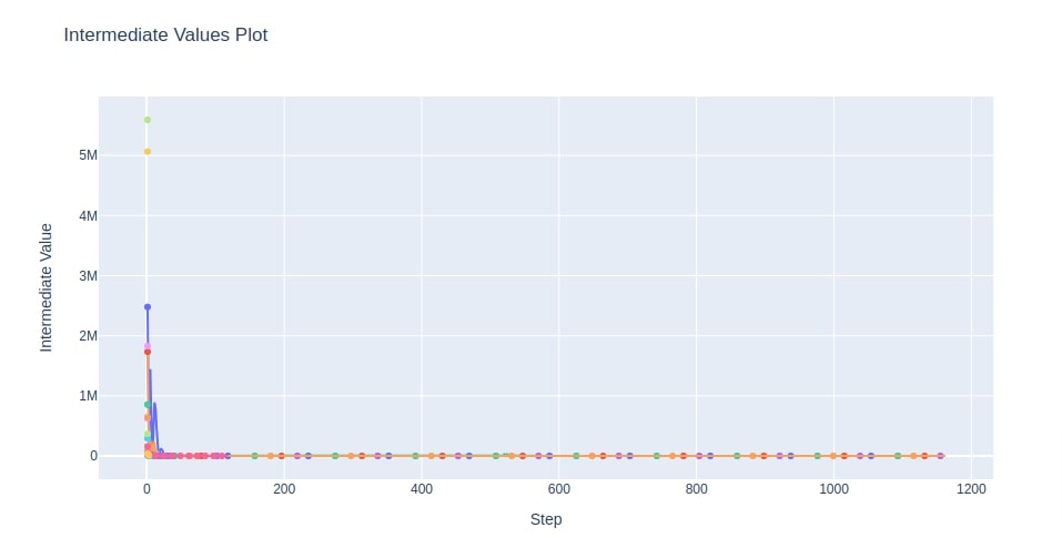
As a part of this section, we'll introduce a chart that shows the progress of all trials on the study process.

This chart shows one line per trial showing how objective value is progressing (increasing/decreasing) during the training process of that trial.

This can be useful to analyze trial progress and why a particular set of trials were pruned. Optuna provides a method named plot_intermediate_values() for the creation of this chart.

• plot_intermediate_values(study) - This method takes as input Study instance and plots chart of lines where each line represents the progress of the individual trial of study. The x-axis of the chart represents a number of steps of the trial and the Y-axis represents the objective value.

The chart will have lines decreasing where we are trying to minimize objective value (MSE) and increasing where we are trying to maximize objective value (Accuracy) over time.

It'll have an entry for some trials till the end of the steps and for some till in between.

The reason behind some of the lines not running all steps of training is because they were deemed underperforming by Optuna and pruned before completion.

Below we have created an intermediate objective values chart of trials using Study object from the multi-layer perceptron section.

7.7 Empirical Distribution Function Plot¶

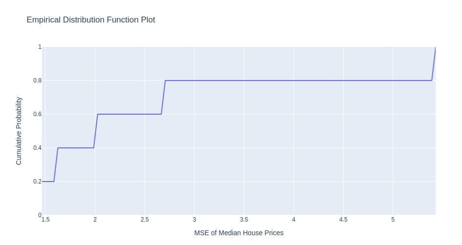
As a part of this section, we'll introduce the empirical cumulative distribution function of objective value.

The chart consists of a single-step line.

The value on the X-axis represents an objective value that we are trying to minimize/maximize and Y-axis represents cumulative probability.

The cumulative probability at any point on the line represents the percentage of trials whose objective value is less than the objective value at that point.

To explain it with an example, let’s say we take a point on the line where cumulative probability is 0.80 and objective value is 2.7. Then of all trials that we tried as a part of the study process, 80% will have an objective value less than 2.7.

• plot_edf(study,target_name='Objective Value') - This method takes as input study instance and creates eCDF chart of objective value.

Below we have created an eCDF chart from Study instance from the multi-layer perceptron section. We can notice that MSE ranges from 0-5+.

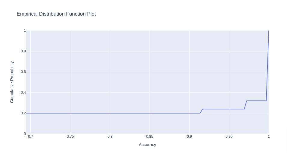
Below we have created eCDF chart of objective value using Study instance from the classification section. The objective value for the classification section was accuracy hence X-axis value ranges in 0-1.

8. Optuna Logging ¶

As a part of this section, we'll introduce few functions which can be used to handle logging messages generated by Optuna.

Optuna by default displays all logging messages of level INFO and above. We can modify this default logging level. Optuna provides two functions for checking and modifying logging levels.

• get_verbosity() - This method returns current set logging level.
• set_verbosity(level) - This method sets new logging level given to it.

If you are interested in learning about logging in python then please feel free to check our tutorial on the same. It tries to explain the topic with simple and easy-to-understand examples.

• Python ""logging" Module Guide

Below we have printed the logging level which is default by optuna. The default logging level is INFO for optuna as we said above.

Below we have modified the logging level to WARNING from INFO. This will now suppress all messages with level INFO and below. It'll now only print all messages with level WARNING and above.

Below we have run our study object from a multi-layer perceptron section for 5 more trials. We can notice now that the info messages about individual trials which were getting displayed earlier are suppressed now.

This ends our tutorial explaining how we can use Optuna with scikit-learn models for hyperparameters tuning. We also covered various visualizations provided by Optuna as a part of this tutorial.

References¶

• Scikit-Learn - Cross-Validation & Hyperparameter Tuning Using GridSearch
• logging - An In-Depth Guide to Log Events in Python with Simple Examples

Other Python Hyperparameters Tuning Libraries¶

• scikit-optimize
• hyperopt
• keras-tuner
• bayes_opt